How To Limit Rows & Columns In Excel & Maximum Number Limit

Managing large Excel spreadsheets can be challenging. Scrolling through endless rows and columns searching for specific information can be frustrating and time-consuming. This is where limiting rows and columns becomes a valuable skill. This can be done through hiding the unwanted rows and columns in Excel Worksheet. Remember, hiding doesn’t delete data, it just removes it from view. You can always unhide rows and columns whenever needed.

Learn how to limit rows and columns in Excel, focusing only on the relevant data for your analysis.

Why To Limit Or Hide Rows & Columns In Excel?

Large Excel spreadsheets can be powerful, but sometimes overwhelming. Endless rows and columns filled with irrelevant data can make it difficult to find what you need. Hiding unused data offers several advantages:

• Focus on what matters: Quickly find the information you need by hiding irrelevant rows and columns.
• Work faster: Navigate through your data with ease, saving time and effort.
• Communicate clearly: Share focused information with colleagues to avoid confusion.

How To Limit Rows And Columns In Excel?

 Here’s how to limit rows and columns, focusing on the information that matters most:

How To Limit Rows In Excel?

You to hide the rows that you don’t want to use without having to delete them. This way, you can still access them if you need to simply by unhiding them. To hide a row in Excel:

• Click the number of the row you want to hide. This highlights the entire row.
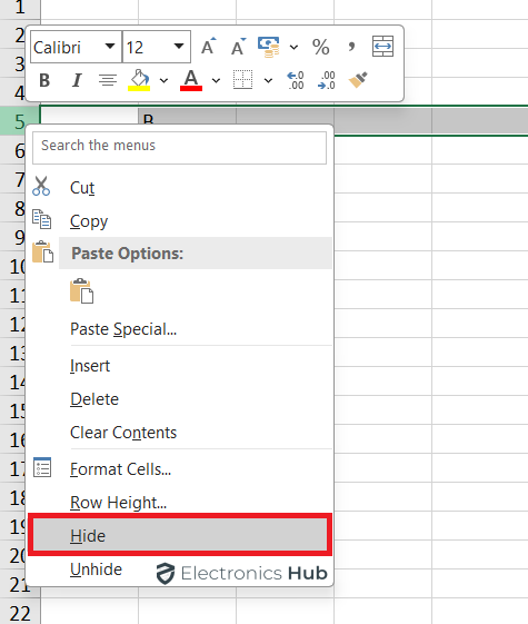
• Right-click anywhere within the highlighted row. A context menu will appear.
• Locate the option labeled “Hide” in the context menu.
• Click on “Hide” to make the row disappear from your view.

How To Limit Columns In Excel?

Here is the process for hiding columns in excel:

• Click the letter at the top of the column you want to hide (e.g., A, B, C). This will highlight the entire column.
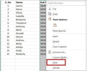
• Right-click anywhere within the highlighted column header.
• A context menu will appear, filled with various options.
• Locate the option labeled “Hide” in the context menu.
• Click on “Hide” to banish the selected column from your view.

How To Unhide Rows And Columns In Excel?

Sometimes, hidden data in your Excel spreadsheet can be just what you need. Here’s a step-by-step guide to bring back those hidden rows and columns:

• Right-click on the row number below the hidden row(s) or the column letter next to the hidden column(s).
• Choose “Unhide” from the menu. The hidden row or column will reappear in its original location.

How To Use Microsoft Visual Basic For Applications Feature

This is a slightly more advanced option in comparison. It allows you to set a scroll area for your worksheet, meaning you can only scroll and select the cells within that area. The rows and columns outside the scroll area will be completely inaccessible.

• To use this method, you need to enable the Developer tab in the ribbon, and then use the VBA editor to enter a code that specifies the scroll area range.
• In the developer tab, click on the “Macros” module and type the name of the function or macro that you wish to execute e.g., Limit_Area and click on the Create button on the right side.
• Now, simply copy the code provided here into the Module(Code) window. Make sure the code is copied above the “End sub” line.
• You can adjust the code as per your requirements. The code snippet provided here limits the scrolling area from A6 to Z20.

ActiveSheet.ScrollArea = “A6:Z20”

• After that, press Ctrl+Q to close the VBA window.
• Now that you are back in the sheet, click on the Macros module again. You will now see the macro you have created.
• Select the macro and click on the “Run” button on the right pane to execute the code.
• Now, your scrolling area will be limited from A6 to Z20.

Note: This is a Temporary Method that will stay active as long as the workbook is open. Once you close the workbook, the method will be reset and activate all of the default rows and columns.

How To Reduce Cells In Excel?

If you want to delete all unused cells in Excel at once, you need to first select the cells that are blank and then delete them together.

1. For that, you can use the Special Go To command to select all the unused cells in a range and then delete them.
2. To do this, first select the range where you want to remove unused cells and then press F5 or Ctrl + G to open the Go To dialog box.
3. Click Special and then select Blanks from the options.
4. Click OK and all the unused cells in the range will be selected.
5. Then, right-click on any of the selected cells and choose Delete.
6. Once deleted, Excel will ask you how to shift the remaining cells to fill the gap in the worksheet.

How To Go To Last Row or Column In A Working Sheet?

There are different ways to check the last row or column in your current worksheet, depending on what you are looking for. With these methods, you will be able to quickly skip to the last cell, row, column, and even the last non-blank cell present in your sheet. Here’s how you can do it:

• To locate the last cell that contains any data or user formatting, click anywhere in the worksheet and press Ctrl+End. This action will move the cursor to the last cell that has been used in the worksheet.
• If you want to select the very last cell in a row or column, you can press End, and then press the Right Arrow key to move to the last cell in the row, or press the Down Arrow key to move to the last cell in the column. This is effective regardless of whether the last cell is blank or contains data.
• For programmatically finding the last non-blank cell in a column using VBA (Visual Basic for Application), you can use the following code:

Dim lastColumn As Long lastColumn = Cells(1, Columns.Count).End(xlToLeft).Column          Columns(lastColumn).Select

• To execute the code, you simply need to create a Macro via the “Macros” option in the developer tab and put the code above “End sub”.
• Then, open the Macros tab again and Run the macro.
• This code starts at the last cell in the first row and goes to the left until it finds the first non-blank cell in that row. The variable lastColumn will hold the column number of the last non-blank cell, and the code then selects the entire column for further actions.

Also check:

• How do I Separate Names  in Excel
• How to Make a Pivot Chart in Ms Excel?
• How To Combine Text In Excel?
• How To Create A Drop-Down List In Excel?
• How To Do Subtract in Excel
• How To Calculate Age in Excel
• How To Move (Swap) Columns In Excel?

What Is The Maximum Limit Of Rows and Columns In Excel?

If you are also using MS Excel as your primary spreadsheet editor, you need to be aware of its current limitations. With that, you can check whether the data you are trying to manage with the tool is compatible with it or not.

1. Worksheet Size

A worksheet can have a maximum of 1,048,576 rows and 16,384 columns.

This means that you can have up to 17,179,869,184 cells in a single worksheet. However, this does not mean that you can use all of them at once. As a matter of fact, the actual number of cells that you can use depends on the available memory and system resources of your computer. If you try to use too many cells, you may experience slow performance, errors, or crashes in the worst-case scenario. As the number of active cells in a spreadsheet increases, it also increases the load on your system. So, it can be beneficial to avoid excessive data entry by limiting the data input, or by limiting the number of rows and columns.

2. Column Width

A column in Excel can have a maximum width of 255 characters.

It indicates that you can display up to 255 characters in a single cell, depending on the font size and type. However, if you enter more than 255 characters in a cell, Excel will still store them. But you will not be able to see them unless you wrap the text or increase the row height to offer additional space. You can counter this limitation by either allotting a different column for mixed data or by increasing the default height of the row so that you won’t have to manage each cell individually.

3. Row Height

An Excel row can have a maximum height of 409.

This means that you can adjust the height of a row to fit the content of the cells up to 409 points. But, if you enter more content than can fit in the row height, Excel will cut off the excess content and display a red indicator in the lower-right corner of the cell.

4. Cell Content

A cell contains a maximum of 32,767 characters that can be either as text, numbers, formulas, or references.

However, only 1,024 characters will be displayed in a cell whereas the rest will be hidden unless you edit the cell or use the formula bar. Also, only 15 digits of a number can be stored in a cell and the rest will be changed to zeros.

5. Page Breaks

An Excel Worksheet has a maximum of 1,026 horizontal and vertical page breaks.

With that, you can divide a worksheet into up to 1,026 pages for printing purposes. If you insert more than 1,026 page breaks, Excel will automatically ignore them and adjust the page layout automatically.

6. Hyperlinks

A worksheet in an Excel can have a maximum of 65,530 hyperlinks in total.

These hyperlinks can be used to redirect to other cells, worksheets, workbooks, web pages, or even files from a single worksheet. If you accidentally insert more than 65,530 hyperlinks, Excel will not create them and display an error message.

Limiting Rows and Columns in Excel – FAQs

How to specify a limited printing section in Microsoft Excel?

To print only a specific section of the Excel worksheet, Excel has a special Print Area feature. It allows users to select a range of cells that they want to print and exclude the rest of the worksheet. Here’s how you can use the Print Area feature:
 
1. Select the range of cells that you want to print. You can do this by clicking and dragging your mouse over the cells, or by typing the cell references in the Name Box.
2. Go to the Page Layout tab in the ribbon, and click the Print Area button in the Page Setup group.
3. Choose Set Print Area from the drop-down menu. You will see a dotted border around the selected range, indicating the print area.
4. Go to the File tab and click Print or press Ctrl + P. Now, you will see a preview of the print area, and you can adjust the settings as needed and then verify the preview again.
5. Once you are sure, click on Print to print the selected section of the worksheet.

Conclusion

Microsoft Excel is a definitely powerful tool that offers numerous features for data management, analysis, and presentation. But, one must understand its capabilities as well as limitations to make sure that it can be used efficiently. One of the common problems that users face while using Microsoft Excel is slower performance or frequent freezes. This happens when there is too much data present in the sheet which overloads your system’s resources. As you can imagine, you will need a powerful machine if you are processing an excessive amount of data. But, there are a few tricks that you can use such as limiting the rows and columns in Excel to improve its performance. In this guide, you will find all the relevant information regarding this problem. If you have any doubt, you can contact us or leave your query in the comment section below.