How To Do Subtract in Excel – Cells, Columns, Dates, Percentages

Let’s be honest, subtracting in Excel shouldn’t be that hard, right? But hey, we’ve all been there – stuck on something that seems super basic.

This guide will have you subtracting like a champ in no time, even when it comes to tricky stuff like dates and percentages. We’ll break things down from the ground up, starting with the simplest subtraction and working our way up. And before we come to a close of this post, we are sure you’ll have all the relevant knowledge, and formulas your spreadsheet throws at you. Here we go.

What Is The Subtraction Formula In Excel?

In Excel, there isn’t a specific “SUBTRACT” function, but that doesn’t mean you can’t perform subtraction. You can use the minus sign (-) arithmetic operator to subtract numbers.

For example, if you have two numbers, 15 and 10, you can enter the formula =15-10 into a cell, and the cell will display 5 as the result.

So, the basic Excel subtraction formula is

= Num1 – Num2.

How To Do Subtraction In Excel?

1. Direct Subtraction

To perform subtraction in Excel, you can use a direct method where you enter numbers manually in a cell and separate them by a minus sign (-) to subtract. Here’s how you can do it:

• Select the cell where you want the result to appear.
• Type the first number.
• Enter the minus sign (-).
• Type the second number.
• Press Enter.

For example, if you want to subtract 16 from 25, you would enter: =25 – 16

And press Enter. The cell will display 9 as the result.

2. Subtract With Reference Cells

Entering each number you want to subtract can be tedious. But if you already have data in cells and want to perform subtraction, you can use those cells instead of entering each number manually. Here’s how you can do it:

Subtract With Two Cells:

• Select the cell where you want the result to appear.
• Type the equal sign (=) to start the formula.
• Click on the cell containing the first number you want to subtract.
• Type the minus sign (-).
• Click on the cell containing the second number you want to subtract.
• Press Enter.

For example, if you have the numbers 15 in cell A1 and 10 in cell B2, and you want to subtract 10 from 15, you would enter: =A1-B2

and press Enter.

Subtract With Multiple Cells:

There are three main ways to subtract multiple cells in Excel:

a. By Using Minus Sign:

• Enter the formula in an empty cell, starting with the equal sign (=).
• Reference the first cell you want to subtract.
• Add minus signs (-) to separate each subsequent cell you want to subtract.
• Reference the remaining cells you want to subtract.

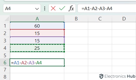
For example, to subtract the values in cells A2, A3, and A4 from the value in cell A1, you would use the formula:

=A1-A2-A3-A4

b. By Using the Sum Function:

To subtract values in a range of cells, use the SUM function to add the cells you want to subtract and then subtract this sum from the minuend.

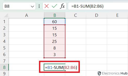
For example, if you want to subtract the sum of cells B2 to B6 from the value in cell B1, you would use the formula:

=B1-SUM(B2:B6)

How To Subtract Columns In Excel?

To subtract columns in Excel row-by-row, you can use a formula and the fill handle. Here’s how:

• Select the Result Cell: Choose the cell where you want the result to appear.
• Enter the Formula: Type the formula to subtract the corresponding cells in each column. For instance, to subtract values in Column B from values in Column A, in cell C1, write =A1-B1.
• Drag the Fill Handle: Move your cursor to the bottom-right corner of the cell with the formula. When the cursor changes to a black plus sign (+), drag it down to copy the formula to the entire column.

Alternatively, you can double-click the plus sign instead of dragging it down to copy the formula to the entire column.

How To Subtract Same Number From A Column Of Numbers?

To subtract the same number from a column of numbers in Excel, you can use a formula with absolute and relative references. Here’s how:

• Enter the number you want to subtract in a cell (e.g., G1).
• Write a formula next to the first number in the column (e.g., B1) to subtract the number in cell G1 from each cell in the column.
• Use absolute referencing for cell G1 to keep it constant in the formula. The formula in cell B1 would be: =A1-$G$1.

• The $ sign in $G$1 indicates an absolute cell reference, locking the number so it doesn’t change when the formula is copied.
• Click on the fill handle (plus sign) of cell B1 and drag it down to fill the formula in the rest of the cells in the column. Excel will adjust the relative references for the cells in the column while keeping the absolute reference to cell G1 constant.

How To Do Subtraction For Percentages In Excel?

To perform subtraction with percentages in Excel, you can use the same methods as discussed earlier for regular numbers. Here’s how:

Subtracting Percentages Directly:

If you have percentages in cells and want to subtract them, you can enter the percentages directly in the formula separated by the minus sign (-).Example:

Cell A1 contains 50%.

Cell A2 contains 20%.

In another cell, enter =A1-A2. The result will be 30%.

Subtracting Percentage from a Number:

If you want to subtract a percentage from a number, you can use the formula =Num * (1 – Percentage/100)

where, Num = number and

Percentage = percentage you want to subtract.

Example: If you want to subtract 20% from 100, you would use the formula =100 * (1 – 20/100), which equals 80.

Remember, when performing calculations with percentages, it’s important to convert them to decimal form (e.g., 20% becomes 0.20) in the formula if necessary. You can also calculate percentage change using subtraction in Excel.

How To Subtract Dates And Time  In Excel?

Subtract Dates

To subtract dates in Excel, simply enter them in individual cells and subtract one cell from the other using the formula:

=Ending date – Starting date

You can also use the DATE or DATEVALUE function to supply dates directly in your formula. For example:

=DATE(2024,4,22)-DATE(2023,4,21) =DATEVALUE(“22/4/2024”)-DATEVALUE(“21/4/2023”)

For more control over the date difference, you can use the DATEDIF function. Its syntax is:

=DATEDIF(start_date, end_date, unit)

Replace start_date and end_date with cell references or actual dates, and specify the unit as follows:

• “Y” for years
• “M” for months
• “D” for days

Example:

=DATEDIF(A2,B2,”D”) (assuming A2 has the start date and B2 has the end date)

Subtract Time

To subtract time, follow a similar approach. Enter the times in individual cells and subtract one cell from the other using the formula:

=Ending Time – Starting Time

Be sure to apply the Time format to the formula cell for the result to display correctly.

You can also supply the time values directly in the formula using the TIMEVALUE function:

=TIMEVALUE(“6:30 PM”)-TIMEVALUE(“1:00 PM”)

How To Subtract Text in Excel?

In Excel, there isn’t a direct function to subtract text from other text. However, you can achieve a similar outcome using a combination of functions. Here’s how you can subtract text in Excel for both case-sensitive and case-insensitive scenarios:

Case-Sensitive Text Subtraction:

To subtract text from one cell from the text in another cell, you can use the SUBSTITUTE function to replace the text to be subtracted with an empty string, and then TRIM the result to remove any extra spaces. For example, if you have “apple” in cell A1 and “le” in cell B1, you can use the following formula:

=TRIM(SUBSTITUTE(A1, B1, “”))

This formula will remove “le” from “apple” and return “app”. If you want to subtract the same text from a range of cells, you can hard-code that text in your formula.

Case-Insensitive Text Subtraction:

For case-insensitive text subtraction, you can use the REPLACE function in combination with the SEARCH and LEN functions. The SEARCH function finds the position of the text to subtract within the original text (ignoring case), which is then used in the REPLACE function to remove that text. For example, if you have “Apple” in cell A1 and “le” in cell B1, you can use the following formula:

=TRIM(REPLACE(A1, SEARCH(B1, A1), LEN(B1), “”))

This formula will remove “le” from “Apple” and return “App”.

FAQs:

Conclusion

Subtracting in Excel goes beyond just using minus signs! This guide shows you its versatility, letting you find the differences in numbers, dates, times, and even text strings. With this knowledge, you can handle a variety of tasks in your spreadsheets, opening up new options for data analysis and manipulation.