Freezing a column or row in Excel keeps it visible as you scroll through the worksheet, making it handy for data comparison. These frozen columns or rows are known as “panes.” This guide will demonstrate how to unfreeze panes in Excel, allowing you to lock specific rows and columns as needed.
Step by Step Guide to Unfreeze Rows and Columns in Excel Sheet
Step 1:- Open a new sheet. or to continue working on your existing sheets, click on “File > Open.” and select a sheet.
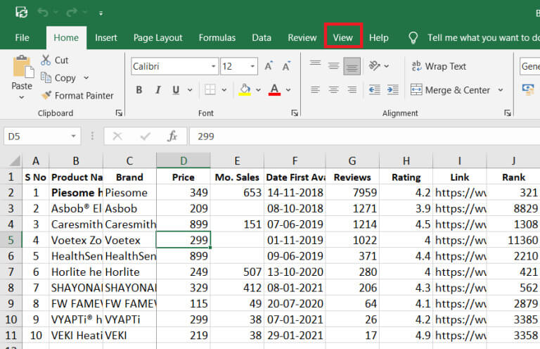
Step 2:- Select view option
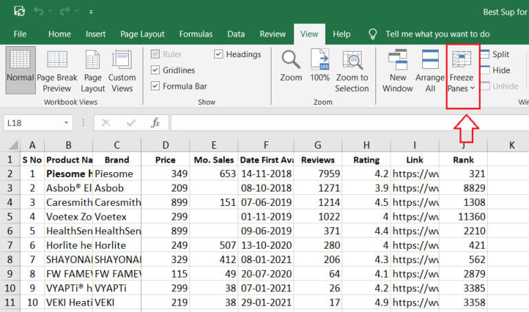
Step 3:- In window section you will find our Freeze Panels click on it
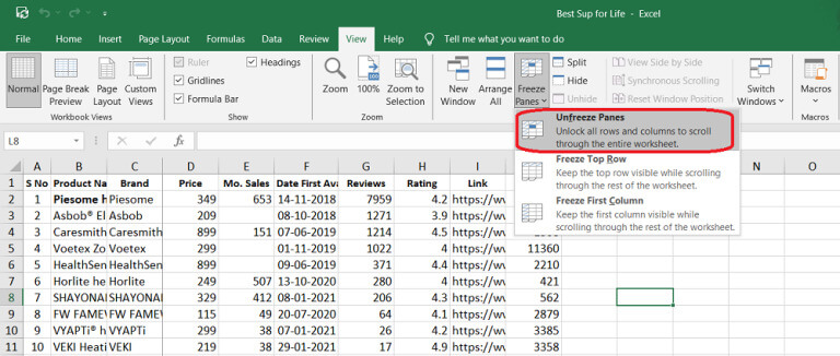
Step 4:- You will see a drop down of 3 options
Step 5:- Click on unfreeze panes Option
Check your sheet by scrolling up and down. You will see that your sheet is unfrozen
FAQs:
Ans: The shortcut to unfreeze cells in Excel is:
1. Press Alt + W to navigate to the View tab.
2. Then press F followed by U to unfreeze the cells.
Ans: Within the “Window” group of the “View” tab, locate the “Freeze Panes” option. Click on “Freeze Panes,” triggering a dropdown menu. From this menu, choose “Unfreeze Panes.” This action will unfreeze any columns previously locked in your Excel sheet, providing flexibility in navigation and data exploration.
Conclusion
In conclusion, our guide on how to unfreeze a column in Excel provides a straightforward approach to maintaining visibility and facilitating data comparison in your worksheets. This user-friendly process ensures a uniform and customized formatting experience, enhancing the overall efficiency of working with Excel sheets.


