How To Create A Drop-Down List In Excel?

Imagine spending hours creating a complex spreadsheet, only to have errors creep in because users accidentally enter the wrong information. Frustrating, right? Drop-down lists are here to save the day!

This powerful Excel feature streamlines data entry, promotes consistency and reduces errors. In this blog post, we’ll walk you through the easy steps of creating a drop-down list, so you can finally ditch the frustration and take control of your data. Keep reading to learn more.

How To Create A Drop-down List In Excel?

Creating a drop-down list in Excel can streamline data entry and ensure consistency in your spreadsheets. There are several ways to create a drop-down list, making it accessible for users to select predefined options. Let’s explore these methods to help you efficiently manage your data

1. Creating A Drop-down List For Small Data

To make a drop-down list in Excel, do the following:

• Select Cells: Select where you want the list. You can choose one cell, many cells, or a whole column. Hold Ctrl to choose multiple non-adjacent cells.

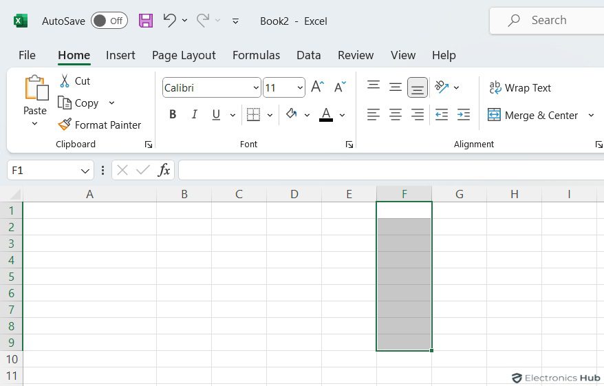
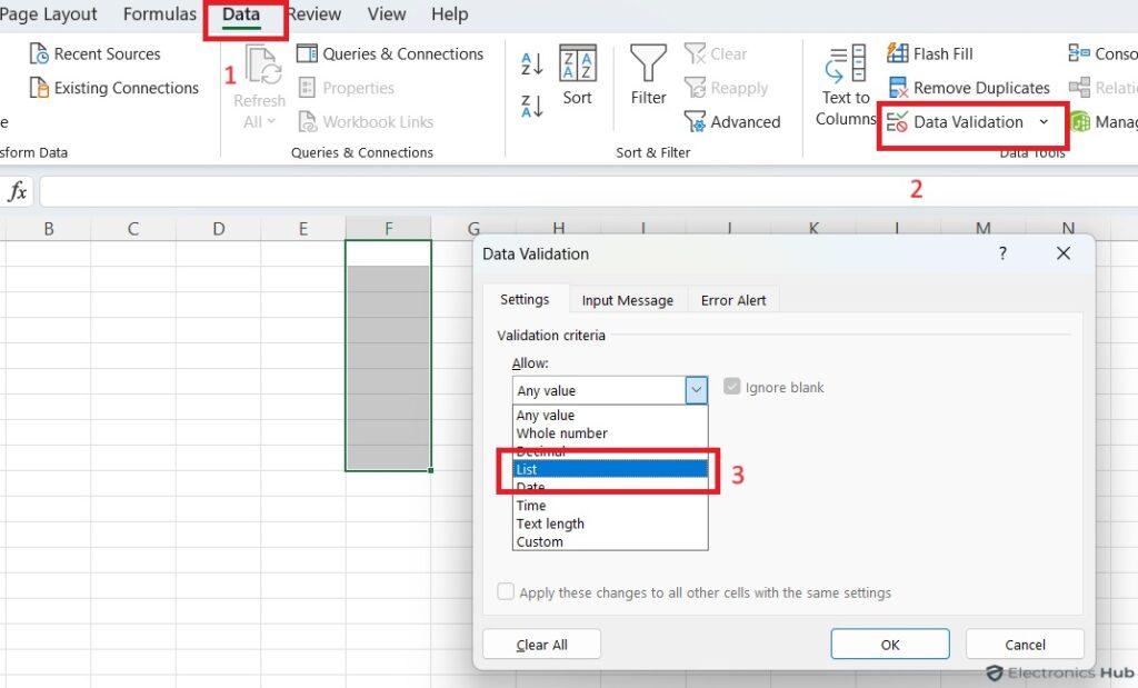
• Open Data Validation: Go to the Data tab. Click “Data Validation” in the Data Tools section.
• Set Up the List: In the Data Validation box, go to the Settings tab. Choose “List” from the Allow menu.

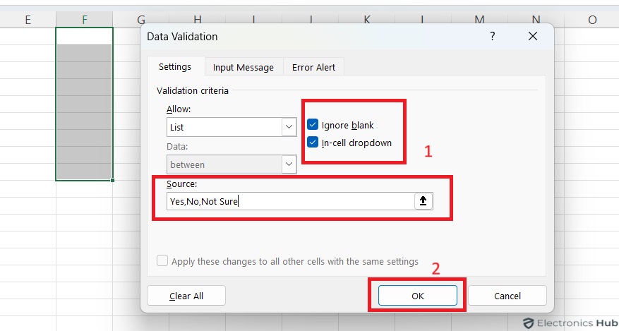
• Enter List Items: In the Source box, type your list items separated by commas. Or, choose a cell range on your sheet with the items.
• Enable Drop-down Arrow: Make sure the “In-cell drop-down” is checked. This shows a drop-down arrow next to your chosen cells.
• Handling Blank Cells: Decide if you want Excel to ignore empty cells in the list.
• Apply Changes: Click OK to finish. Your drop-down list is ready to use!

That’s all! You’ve made a drop-down list in Excel.

Note: For small data validation lists that are unlikely to change, a drop-down list of comma-separated values is suitable. However, for frequently updated lists, it’s better to use a range or table as the source. Below are detailed step-by-step instructions for each method.

2. Creating A Drop-down List From Range

Creating a drop-down list in Excel based on a range of cells is a smart way to keep your data consistent and easy to manage. Here’s how you can do it:

• Type each item for the list in separate cells, either in the same worksheet or a different one.
• Select the cell or cells where you want the drop-down list.
• Go to the “Data” tab, then click “Data Validation” in the “Data Tools” group.
• In the “Data Validation” dialog box, choose “List” from the “Allow” drop-down menu.
• In the “Source” box, select your range of cells:
• Click and drag to select the cells.
• Alternatively, Click the collapse dialog icon and choose the range.

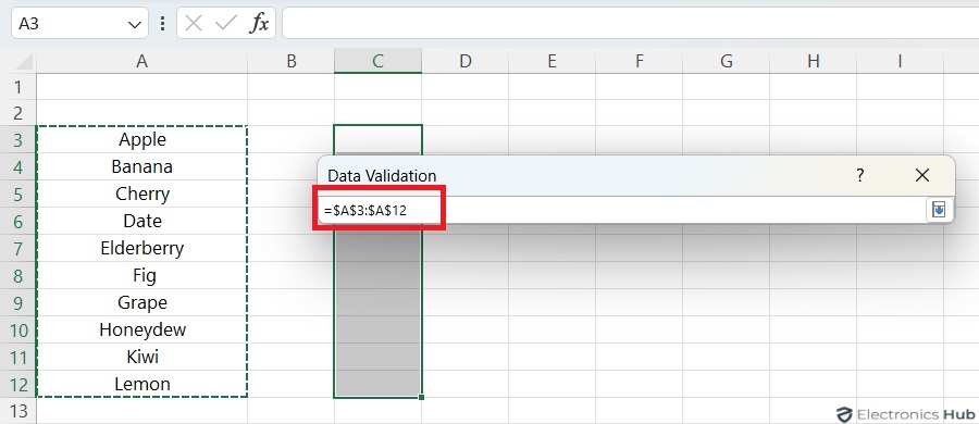
• Click “OK” to close the dialog box.
• Now, you’ll see a small arrow in the cell. Click it to see and select items from your list.

3. Creating A Drop-down List From The Named Range

Creating a drop-down list in Excel from a named range is a handy way to manage your data efficiently. While the initial setup may take a bit of time, it can save you considerable effort, especially if you need to update the list frequently. Here’s how to do it:

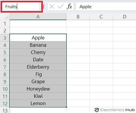
• Prepare Your List: List the items you want in your drop-down list in a single column or row on your worksheet, ensuring there are no blank cells between them.
• Define a Named Range: Select all the cells containing your list items. In the Name Box at the top left corner of the Excel window, type a clear and descriptive name for your list and press Enter to finalize the named range.

• Select the Cell(s) for the Drop-Down List: Choose the cell or range of cells where you want the drop-down list to appear.
• Access Data Validation: Go to the “Data” tab on the Excel ribbon. In the “Data Tools” group, click on “Data Validation.”
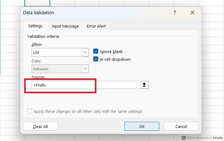
• Configure Data Validation: In the “Data Validation” dialog box, select “List” from the “Allow” dropdown menu. In the “Source” box, type an equal sign (=) followed by the name you assigned to your list in step 2.

• Finalize Drop-down List Settings: By default, a small arrow will appear next to the cell to indicate the drop-down list. Ensure the “In-cell dropdown” checkbox is selected. Optionally, check the “Ignore blank” box if users can leave the cell empty. Uncheck it to require a selection from the list.
• Apply and Confirm: Once you’ve configured the settings, click “OK.”

4. Creating A Drop-down List From Excel Table

Instead of using a named range, you can put your data into an Excel table. When your data is in a table, any drop-downs you create based on that table will update automatically as you add or remove items. Here’s how you can set it up:

• Enter your list of items into a table. You can type the list directly into a table or convert an existing range to a table using the Ctrl+T shortcut.

• Choose the cell or range of cells where you want the drop-down list to appear.
• Go to the “Data” tab on the Excel ribbon.
• In the “Data Tools” group, click on “Data Validation.”
• In the “Data Validation” dialog box, select “List” from the “Allow” dropdown menu.
• In the “Source” box, reference the entire table using a structured reference.
• Check the “In-cell dropdown” box to show the drop-down arrow in the cell. If it’s okay for the cell to remain empty, check the “Ignore blank” box.
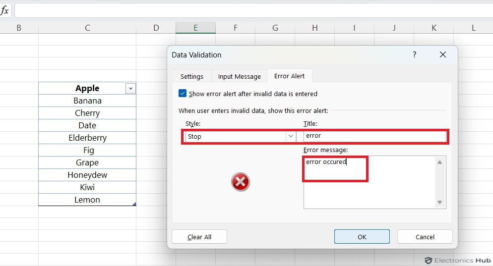
• Then switch to the “Error Alert” tab in the “Data Validation” dialog box.
• Check the “Show error alert after invalid data is entered” box if you want a message to pop up when an invalid entry is made.
• Choose an option from the “Style” dropdown, and enter a title and message.
• Once you’ve configured the settings, click “OK.”

How To Create Different Types Of Drop-down Lists In Excel?

Once you know how to create a basic drop-down list in Excel, you can explore different types to suit your needs. Here are a few variations:

1. Dynamic Drop-down List

If you often change your picklist items, it’s best to create a dynamic drop-down list. This type of list updates automatically in all cells whenever you add or remove items from the source list.

The quickest method to create a dynamic drop-down in Excel is by using a table which explained above

Another approach is to use a regular named range and reference it with the OFFSET formula, as explained below.

Step 1: Enter Items for the Drop-down Menu

Start by typing the items you want in the drop-down menu in separate cells, like A2 to A10.

Step 2: Define a Named Range

• Select the cells with your items (e.g., A2:A10).
• Go to the “Formulas” tab, click “Name Manager,” and then “New.”
• Give your range a name (e.g., “Fruits”), and in the “Refers to” box, enter:

=OFFSET($A$2,0,0,COUNTA($A$2:$A$10),1)

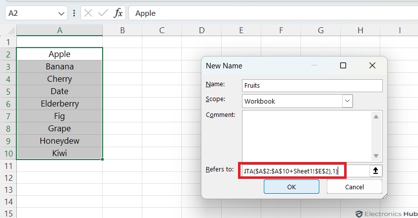
• Click “OK.”

Step 3: Create a Dropdown List

• Select the cell where you want the dropdown.
• Go to the “Data” tab, click “Data Validation,” and choose “List.”
• In the “Source” box, type your named range (e.g., “=Fruits”).
• Click “OK.”

Now, your Excel dropdown list will update automatically as you add or remove items in column A.

2. Drop-down List With Color

In Excel, you can create a drop-down list with colors using a combination of conditional formatting and data validation. Here’s how you can do it:

Creating the Drop-down List:

This allows users to choose from a predefined list, which is explained earlier.

Applying Conditional Formatting:

This adds visual cues by assigning colors to specific options within the drop-down list. Here’s how:

• Select Cells: Highlight the cell(s) with the drop-down list.
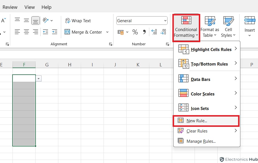
• Open Conditional Formatting: Go to the Home tab, and click Conditional Formatting.
• Set Up Color Rules: Choose a New Rule.

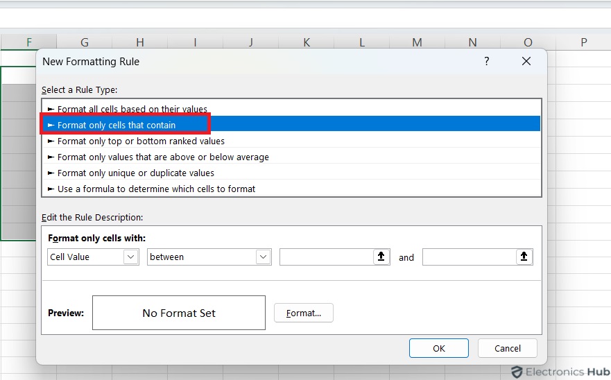
• Format Based on Selection: Select “Format cells that contain” in the “New Formatting Rule” dialog box.

Define Color Condition:

• Choose “Specific Text” from the first drop-down.
• Select “containing” from the second drop-down.
• Enter the item text (e.g., “Red“) in the third box.
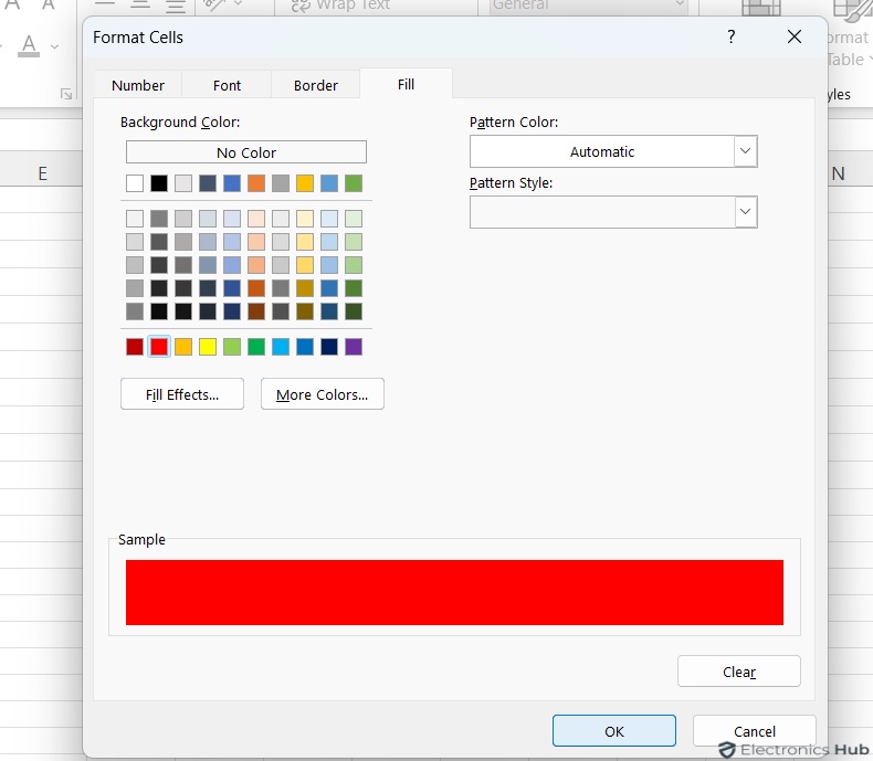
• Set Color Format: Click Format, choose the fill color under the Fill tab in the “Format Cells” dialog box. Click OK twice.

• Repeat for Other Colors: Repeat steps 4-6 for different list items/colors.

Result: The selected cell will be highlighted with the color assigned to the chosen item from the drop-down list.

3. Searchable Drop-down List

Excel 365 offers a convenient built-in feature for searchable drop-down lists, eliminating the need for complex workarounds. Here’s how to utilize it:

Create the Drop-down List:

Follow the steps mentioned previously on how to create a drop-down list. You can define the list items by typing them directly, selecting a range of cells containing the list, or using a named range.

Use AutoComplete:

• After creating the list, click the cell with the arrow.
• Start typing the first letters of the item you want.

Excel 365’s AutoComplete feature will automatically filter the list as you type. Matching options will appear, narrowing down the choices as you enter more characters. This makes it much faster to find specific items in large drop-down lists.

How To Create A Drop-down From Another Worksheet?

To make a drop-down menu in Excel that fetches data from another worksheet, you have three options: normal range, named range, or Excel table:

• Named Range: Set the name’s scope to the current workbook, then create a data validation list as usual.
• Excel Table: No extra steps are needed, as table names/references work across the entire workbook.
• Normal Range: Include the sheet’s name in the source reference. In the Data Validation dialog, click in the Source box, switch to the other sheet, and select the range with the items. Excel will automatically add the sheet name to the reference.

How To Insert A Drop-down From Another Workbook?

Inserting a drop-down list from another workbook in Excel might seem tricky, but you can achieve a similar result using named ranges. However, remember that this method requires the source workbook to be open for the drop-down list to work, and any changes made to the source list won’t automatically update in the drop-down list. Here’s how to do it:

Create a Named Range in the Source Workbook:

• Open the workbook with the list you want to use.
• Select the cells with your list items.
• Go to the “Formulas” tab, click “Name Manager,” then “New.”
• Name your range (e.g., “Colors”) and specify the range reference (e.g., A1:A5).

Define a Name in the Main Workbook:

• Open the workbook where you want the drop-down list.
• Go to the “Formulas” tab, click “Name Manager,” then “New.”
• Name your reference (e.g., “Color“) and in the “Refers to” field, enter:='[Source Workbook.xlsx]Sheet1′!Colors

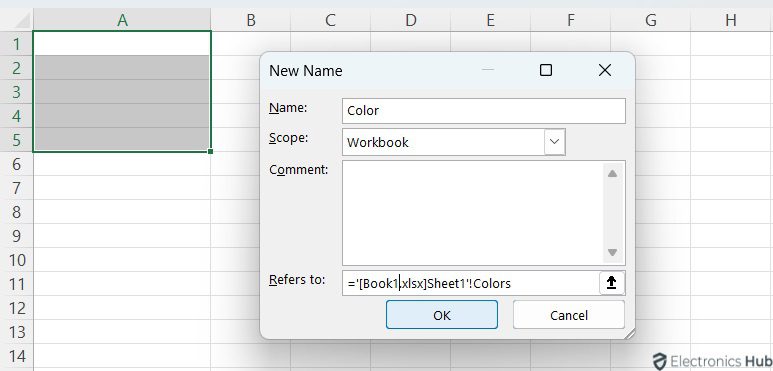
Replace “Source Workbook.xlsx” with your source workbook’s name and “Sheet1” with the sheet name containing your named range.

Create the Drop-down List:

• Select the cell(s) for the drop-down list.
• Go to the “Data” tab, click “Data Validation,” and choose “List.”
• In the “Source” box, enter the name you defined in the main workbook (e.g., “=Color”).
• Click “OK” to save.

Now, whenever you open the main workbook, the drop-down list will display items from the named range in the source workbook, as long as the source workbook is open.

How To Insert A Drop-down List With Message?

When creating a drop-down list in Excel, you can add an informative message that shows up when the cell is selected. This helps provide instructions or more context. Here’s how:

• Click on the cell where you want the drop-down list.
• Go to the “Data” tab and click “Data Validation.”
• In the “Data Validation” dialog, choose “List” from the “Allow” menu. Enter your list items’ range in the “Source” box.
• Go to the “Input Message” tab.
• Check “Show input message when cell is selected.”
• Enter a title (e.g., “Instructions“) in the “Title” box.
• In the “Input message” box, type your message (up to 225 characters).
• Click “OK” to save and close.

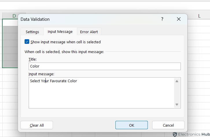
Now, clicking the cell with the drop-down list will display your message, offering guidance or information about the list.

How To Add Or Remove An Item From An Existing Drop-down List In Excel?

Adding or removing items from an existing drop-down list in Excel can be done in two main ways, depending on how the list was created:

1. Modifying the Source List:

• Click on the cell with the drop-down list.
• Find and open the range of cells with the source list (usually on the same sheet).
• To add an item, type it at the end of the list.
• To remove an item, select the entire row with the unwanted item and press Delete.
• Ensure that the Data Validation settings in the target cell (with the drop-down list) reference the correct cell range for the updated source list.

2. Modifying a Named Range:

• Go to the Formulas tab.
• Click on Name Manager in the Defined Names group.
• Find the named range for your drop-down list and select it.
• Click in the Refers to the box.
• Modify the cell range to reflect the updated source list, including new items or excluding removed ones.
• Save the changes to the named range.

You can also add or remove items from a drop-down list directly without opening the ‘Data Validation‘ dialog box and changing the range reference:

• To add an item, right-click on an item in the list, click “Insert,” select “Shift cells down,” and then type the new item.
• To remove an item, right-click on the item, click “Delete,” and select “Shift cells up.“

Excel will automatically adjust the range reference. You can verify this by opening the ‘Data Validation’ dialog box.

How To Remove Drop-down List In Excel?

There are two main ways to remove a drop-down list in Excel, depending on whether you want to simply clear the list selection or completely remove the functionality:

1. Clear the Drop-down List Selection:

If you only want to remove the current selection from the drop-down list and allow users to choose another option:

• Click the Cell: Select the cell containing the drop-down list.
• Delete Selection: Press Delete or Backspace to clear the current selection from the drop-down list. The cell will remain blank, allowing users to choose a new option from the list.

2. Remove Drop-down List Functionality:

If you want to completely remove the drop-down list functionality from the cell:

• Select the Cell: Click on the cell containing the drop-down list.
• Open Data Validation: Navigate to the Data tab and click Data Validation in the Data Tools group.
• Clear All Settings: In the “Data Validation” dialog box, click the Clear All button on the Settings tab.

• Click OK: Click OK to confirm the removal of the drop-down list settings from the cell.

The cell will no longer have drop-down functionality and will behave like a standard text cell.

FAQs:

Conclusion

In short, incorporating drop-down lists into your Excel spreadsheets is a powerful way to enhance both usability and efficiency. These lists not only streamline data entry and minimize errors but also offer flexibility in creation, allowing you to source data from various ranges or tables. Whether you’re working with inventory, expenses, or any other data organization task, drop-down lists can significantly improve your workflow. So, why not start incorporating them today?