How To Calculate Percentage Change in Excel? A Step-by-Step Guide

Confused by numbers in your spreadsheets? You’re not alone!

Numbers are everywhere, but what do they really tell you? Percentages are the key to unlocking the secrets of your data, like growth trends and performance changes. But who wants to crunch numbers manually? Not you!

This guide is here to save the day (and your sanity). We’ll show you a super easy Excel formula that calculates the percentage change in a flash, with step-by-step instructions.

What Is Percentage Change In Excel?

Percentage change in Excel shows the relative change between two values as a percentage. It’s used in finance, stats, and other fields to understand how a value has changed over time or between situations.

Percentage Change = (New Value−Old Value/ Old Value) ×100

This formula subtracts the old value from the new value in Excel to find the difference, then divides that difference by the old value (A1) to find the ratio of change, and finally multiplies by 100 to express the change as a percentage.

How Do You Calculate Percentage Change In Excel?

Excel provides two valuable methods to determine the change between two values as a percentage. These methods are ideal for analyzing changes in sales figures, stock prices, or any other numerical data.

Method 1 – Calculate Percentage Change

This method breaks down the calculation into two steps: finding the difference and then converting it to a percentage relative to the original value.

Formula = ((New Value – Old Value) / Old Value) * 100

Steps to Calculate the percentage of change between two numbers

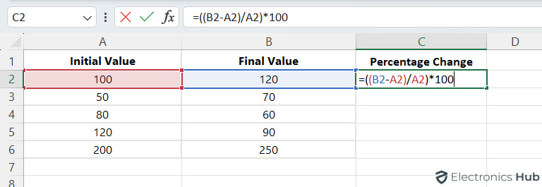
• Identify the Values: Choose the old and new values. Let’s say the old value is in cell A2, and the new value is in cell B2.
• Calculate the Difference: Subtract the old value from the new value in a new cell using the formula: =B2-A2.
• Find the Ratio: Divide the difference by the old value with the formula: =(B2-A2)/A2.
• Convert to Percentage: Multiply the ratio by 100 to get the percentage change: =((B2-A2)/A2)*100

Alternatively, you can use a slightly easier method

Method 2 – Calculate Percentage Change 

This method uses a single formula to achieve the same result as Method 1 in a more concise way.

Formula = ((New Value / Old Value) – 1) * 100

Here’s how you can calculate percentage change by using this method:

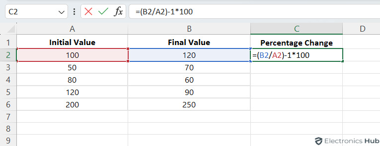
• Divide the New Value by the Old Value: = B2/A2
• Subtract 1 from the Quotient: = (B2/A2) – 1
• Multiply by 100 to Convert to Percentage Form: = ((B2/A2) – 1)*100

What Is The Percent Change Keyboard Shortcut In Excel?

While Excel lacks a specific keyboard shortcut for directly calculating percentage change, you can achieve this efficiently using two reliable methods. Choose the formula that best suits you (refer to our previous explanation of Method 1 and Method 2).

Formatting as a Percentage (Shortcut):

• Calculate the change using a formula.
• Select the cell with the result.
• Press Ctrl + Shift + % or Alt + H + P.
• This shortcut formats the cell as a percentage, automatically converting the decimal value to a percentage with the correct symbol.

Formula with Function Key (Optional):

• Enter the percentage change formula in the formula bar for the first cell.
• Copy the formula to other cells with your data.
• While copying, press F4 before each cell reference (e.g., A1) to lock those references. This ensures the formula uses the correct relative positions as you copy it across the spreadsheet.

How To Calculate Percent Change Between Multiple Sets Of Data?

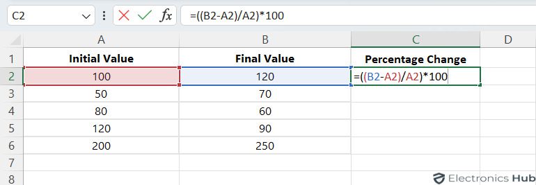
• Enter the Values: In Excel, put the old values in one column (like column A) and the new values in another column (column B).
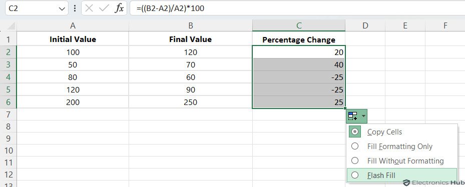
• Calculate the Percentage Change: In a new column (column C), use the formula =((B2-A2)/A2)*100 to calculate the percentage change for each set of data. Then multiply by 100 to show the change as a percentage.

• Autofill the Formula: After entering the formula in the first cell of column C, you can autofill the formula down the column to calculate the percent change for all the data sets.

How To Calculate Percent Increase and Decrease In Excel – Examples

Percentage change can go up or down, indicating either growth or decline. A positive change means things are on the rise, while a negative one suggests a drop. We’ll use the same math for both situations, but what they mean will be different.

Here’s the formula: = (New Value – Old Value) / Old Value

Let’s break it down for positive and negative results:

• For a positive result, like 0.1, it’s a percentage increase.
• For a negative result, like -0.2, it’s a percentage decrease.

Let’s check out two examples:

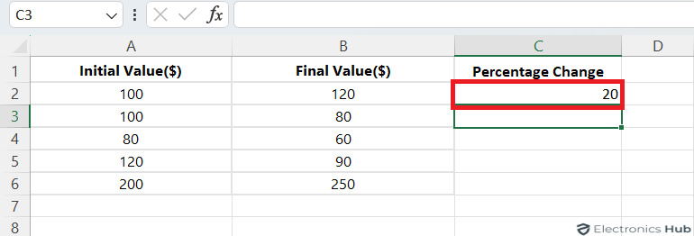
Example 1: Price Increase

Old price (A1): $100

New price (B1): $120

Calculate the percentage change in cell C1: = (B2-A2)/A2 = (120-100)/100 = 0.2

Convert to percentage in cell D1: = ((B2-A2)/A2) * 100 = (0.2 * 100) = 20%

Interpretation: The price has increased by 20%.

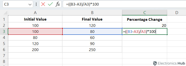
Example 2: Sales Decrease

Old sales (A3): 100 units

New sales (B3): 80 units

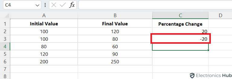
Calculate the percentage change in cell C1: = (B3-A3)/A3 = (80-100)/100 = -0.2

Convert to percentage in cell D1: = ((B3-A3)/A3) * 100 = (-0.2 * 100) = -20%

Interpretation: Sales have decreased by 20%.

How To Use Percentage Change In Excel For Various Scenarios?

Excel’s percentage change function applies to numerous scenarios. Let’s explore some common use cases:

1. Calculate Percentage Change Over Time in Excel

To calculate percentage change in Excel, you can use either the simple percentage difference or the Compound Annual Growth Rate (CAGR) method, depending on your needs.

Simple Percentage Difference:

• Identify Old and New Values: Select the two values you want to compare, like the old value in cell A1 and the new value in B1.
• Calculate Percentage Change: Subtract the old value from the new value, then divide by the old value, and multiply by 100. The formula is: =((B1-A1)/A1)*100

Example:

Old Value (2019): $100

New Value (2020): $120

Percentage Change: =((120-100)/100)*100 = 20%

Compound Annual Growth Rate (CAGR):

• Identify Beginning and Ending Values: Pick the initial (beginning) and final (ending) values over a period.
• Calculate CAGR: Use the formula: CAGR = (Ending Value/Beginning Value)^(1/Number of Years) – 1

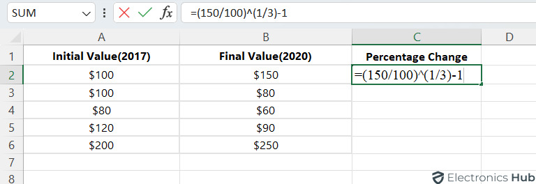
Example:

Beginning Value: $100 (2017)

Ending Value: $150 (2020)

Number of Years: 3

CAGR: =(150/100)^(1/3) – 1 ≈ 14%

These methods offer different perspectives on change over time, with the simple percentage difference showing the change between two points and CAGR providing an average annual growth rate over periods.

2. Calculate Percent Change Absolute Value in Excel

In financial analysis or when comparing trends, it’s important to measure the size of change between two values, regardless of whether it’s an increase or decrease. Calculating the absolute value of percentage change in Excel helps with this.

Formula: Excel’s ABS function is used for this calculation. The formula is:

= ABS((New Value – Old Value) / Old Value) * 100

Example: Let’s say you’re analyzing price changes:

Old price (A2): $100

New price (B2): $120

Calculate Absolute Percentage Change:

In cell C1, enter the formula: = ABS((B2-A2)/A2) * 100

This will calculate: = ABS((120-100)/100) * 100 = 20%

Interpretation: The price has changed by 20%, indicating a 20% increase.

3. Calculate Discount Percentage

Discounts play a crucial role in sales and marketing strategies. Excel makes it easy to calculate the discount percentage on an original price, helping businesses make informed decisions about pricing and profitability.

Formula for discount percentage: There are two main approaches:

1. Direct Comparison:

Formula: = (Discounted Price – Regular Price) / Regular Price

Example: Let’s say a shirt with a regular price of $50 (say cell A2) is on sale for $40 (say cell B2). What’s the discount percentage?

Enter the formula = (B2-A2)/A2 in a new cell (say, C2).

Result: = (40-50)/50 = -0.2 (or -20%)

2. Shorter Formula:

This method uses a single formula to achieve the same result:

Formula: = Discounted Price / Regular Price – 1

Note: These formulas result in negative values (discounts decrease the price). To display a positive percentage, use the ABS function:

= ABS((Discounted Price – Regular Price) / Regular Price)

Example (using ABS function):

In the same scenario (shirt price), enter the formula = ABS((C2-B2)/B2) in another cell (say, E2).

Result: = ABS((40-50)/50) = 0.2 (or 20%)

Interpretation: The discount is a positive 20%, reflecting the percentage decrease from the regular price.

How To Calculate The Value After Percent Change In Excel?

Calculating final values after percentage changes in Excel is handy for various tasks like discounts, growth projections, or analyzing price shifts. Here’s a simple guide:

Formula: = initial_value * (1 + percent_change)

initial_value: Original value before the change (e.g., cell B2).

percent_change: Change percentage in decimal form (e.g., cell C2). Positive for increase, negative for decrease.

Steps:

• Organize Your Data: Put original values in one column (e.g., column B) and corresponding percentage changes in another (e.g., column C).
• Calculate Final Values: In a new column (e.g., column D), put the formula =B2*(1+C2) in the first cell (D2).
• Copy this formula down to other cells in column D to apply to all data.

Example:

Let’s say you have product prices in B and discount rates in C. You want to find final discounted prices in D.

Product Price (B2): $100

Discount Rate (C2): -10% (as -0.1 in the formula)

Final Discounted Price (D2):

Enter =B2*(1+(C2/100)) in D2.  To convert a percentage to a value, divide the percentage by 100.

Calculation: $100 * (1 – 0.1) = $90.00

Interpretation: The final price is $90.00, reflecting a 10% decrease.

Alternatively,

• You can input percentage changes directly in the formula.
• To increase all values in column B by 5%, use =B2*(1+0.05) in D2 and copy it down.
• For convenience, define a cell (e.g., G2) for the percentage change. Then, reference it in the formula using absolute cell references (e.g., =B2*(1+$G$2)) to easily adjust the change for the whole column by modifying G2.

How To Calculate Percent Change With Negative Values In Excel?

Calculating percent change in Excel can be confusing, especially with negative numbers. However, there’s a simple trick to make it easier:

• Instead of dividing by the original negative number, use the ABS function to make it positive. ABS turns any number positive, even negatives.
• Then, apply the regular percent change formula: (New Value – Old Value) / ABS (Old Value).

Example:

Let’s consider inventory (in negative numbers):

Before (A1): -50 units (negative, meaning you owe 50 units)

Now (B1): -20 units (negative, meaning you owe 20 units)

What’s the percent change in inventory?

Step 1: Find the Absolute Value

Ignore the negative signs. Just focus on the difference between the two amounts owed. So, pretend A1 is 50 and B1 is 20.

Step 2: Use the Regular Formula

Now, use the regular formula:

= (New Value – Old Value) / ABS (Old Value)

= (-20 – (-50)) / 50 (Plug in the numbers without negative signs)

= 30 / 50

= 0.6 (or 60%)

Your inventory has actually increased by 60% (even though the numbers are negative). This means you owe 60% less than before.

Note: Be aware that while the ABS adjustment formula is technically accurate, it can lead to misleading outcomes when the original value is negative and the new value is positive, or vice versa.

How To Handle The #Div/0 Error When Calculating Percentage Change?

Encountering a #DIV/0 error in Excel usually means you’re trying to divide by zero. This often happens when calculating percentage change, especially if your data contains zero values. Here are two simple ways to deal with this issue:

Method 1: Using IF Functions

The IF function helps you set conditions in your formula. Here’s how:

=IF(B2=0, 0, (B2-A2)/A2) * 100

(B2 is the new value, A2 is the old value)

Explanation:

• IF checks if the new value (B2) is zero.
• If it is, the formula returns 0 to avoid the error.
• If not, it calculates the percentage change normally and multiplies by 100 for the percentage.

Method 2: Using IFERROR Function

IFERROR allows you to handle errors gracefully. Here’s how:

=IFERROR((B2-A2)/A2 * 100, “Error: Division by Zero”)

(B2 is the new value, A2 is the old value)

Explanation:

Attempts the regular calculation.

If an error occurs (like #DIV/0), it shows “Error: Division by Zero” instead.

Choosing the Right Method:

Method 1: Good if you want to replace the error with a specific value (like 0) when the new value is zero.

Method 2: Useful for displaying a clear error message when encountering a #DIV/0 error.

Note: You can change “Error: Division by Zero” in Method 2 to any message you want.

Benefits Of Using Percentage Change In Excel

Analyzing trends over time is easier with Excel’s percentage change feature. Whether it’s sales figures, website traffic, or other data, this tool offers valuable insights. Here are some benefits of using percentage change in Excel:

• Standardized Comparison: Percentage change helps compare data sets easily, making interpretation and analysis simpler.
• Easy Trend Identification: Calculating percentage change allows quick identification of trends, like growth or decline over time.
• Normalized Data: Percentage change normalized data, aiding in comparing values on different scales.
• Effective Visualization: Percentage change is easily visualized using charts or graphs, aiding in communicating trends to others.
• Decision Making: Understanding percentage change assists in making informed decisions based on data trends and patterns.

Tips To Quickly Calculate Percentage Change In Excel

• Use Cell References: Instead of typing values directly, use cell references. This makes it easier to copy formulas and ensures they update automatically if the data changes.
• Consider Absolute Cell References: For formulas you’re copying across rows but want the initial value reference to remain constant, use absolute cell references (e.g., $A).
• Format Result Cells: Format cells containing percentage change results as percentages for easier interpretation.
• Utilize Named Ranges: Instead of manually selecting cells, use Excel’s named range feature to reference cells quickly and accurately.
• Create Templates: If you often calculate percent change for similar data, create a template as a starting point to save time.
• Explore Macros: Macros can automate repetitive tasks like formatting or copying and pasting data, making your workflow more efficient.

Troubleshooting Common Errors With Calculating Percent Change In Excel

When you calculate percentage change in Excel, you might run into a few common problems. Here’s how to fix them:

• Divide by Zero Error (#DIV/0): This happens when the old value is zero, causing a division by zero error. To solve this, use an IF statement to check if the old value is zero. For example, use =IF(A1=0, “N/A”, ((B1-A1)/A1)*100).
• Incorrect Cell References: Make sure you’re referencing the correct cells in your formula. Check the cell references to ensure they match the old and new values.
• Incorrect Formula Syntax: Double-check that your formula is entered correctly. Use the right operators (+, -, *, /) and parentheses where needed.
• Formatting Issues: If your percentage change values aren’t showing up correctly, check the cell formatting. Select the cells and apply the percentage format to display them correctly.
• Data Type Issues: Confirm that the old and new values are formatted as numbers. If they’re formatted as text, Excel might not calculate the percentage change correctly.

FAQs:

Conclusion

No more staring at spreadsheets confused. These easy formulas and the steps mentioned will have you analyzing data like a champ. Feel free to bookmark this post in case you ever forget the magic trick (but you probably won’t). Thanks for reading.