In contrast to the electrostatics, which deals with static electric charges (also called Coulombian approach), magneto statics deals with stationary electric currents (also called Amperian approach). In 1820, the scientist Oersted has discovered the relationship between electric and magnetic fields.
He stated that the charges are surrounded by a magnetic field when charges are in motion. Hence, the current carrying conductor is always surrounded by a magnetic field. If a steady or time invariant current flows through a conductor, a steady magnetic field is produced around the conductor.
This steady current is nothing but a direct current (DC). Thus, a study of steady magnetic fields due to steady or direct current is called as magnetostatics.
what is Magnetostatics?
Magnetostatics is the study of magnetic fields in systems where the electrical currents are constant or steady over time. This field of physics examines the magnetic forces, fields, and effects produced by steady (unchanging) currents, providing a foundation for understanding and designing various electrical devices and systems that rely on magnetic interactions under static conditions.
Fundamentals of Magnetic Fields
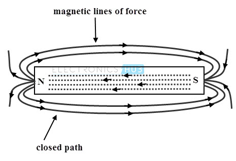
Before learning fundamental concepts of magnetic fields, let us understand the basic properties of the magnetic fields. Consider a permanent magnet that has two poles namely North (N) and South (S). The region within which the influence of a magnet is experienced around the magnet is called as a magnetic field.
This field is nothing but a representation of imaginary lines around the magnet which are also called as magnetic lines of force or magnetic flux lines. Famous English scientist Michael Faraday has introduced such lines and its direction is from north to South Pole, external to the magnet.
The magnetic flux lines always exist in the form of a closed loop; that means the flux lines starting from N pole must be terminated at S pole irrespective of the field i.e. either due to the current carrying conductor or due to permanent magnet.
Magnetic Field Produced by Electric Current
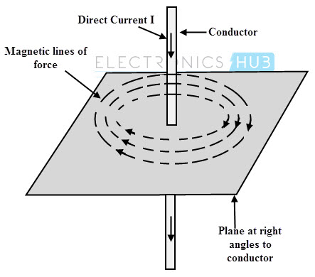
As we know that electric charges in motion constitute an electric current and also such charges in motion produces a magnetic field. Consider that a current of I ampere (DC) is flowing in a straight conductor. Then it produces a magnetic field around the conductor all along the length of the conductor directed along a circle in a plane normal to the current.
These lines of force are in the form of concentric circles in the plane right angles to the conductor. The direction of these lines of force depends on the direction of current through the conductor. A steady magnetic field is produced around the conductor as long as the constant and time invariant current is flowing through the conductor.
The direction of magnetic field is determined by the right handed screw rule. In this method, the direction of magnetic field is given by the direction of right handed screw that will have to be turned to make it progress in the direction of current.

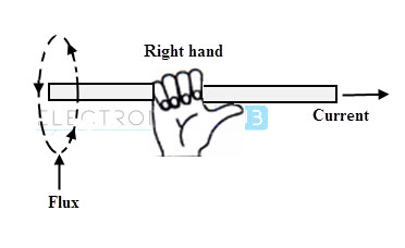
Another easy way to determine the direction of magnetic field is the right hand thumb rule. It states that, if we hold the conductor in the right hand with thumb pointing in the direction of current and parallel to the conductor. Then, the curled fingers of the right hand give the direction of the magnetic field around the conductor.
Magnetic Flux Density
The magnetic flux density is denoted as B ̅ and is defined as the total magnetic lines of force or the magnetic flux per unit area in a plane that is perpendicular to the direction of the magnetic field.
It is a vector quantity and is measured in Weber per meter square (Wb/m2) also called as Tesla (T).
Magnetic Field Intensity
The magnetic field strength or magnetic field intensity gives the quantitative measure of weakness or strongness of the magnetic field. It is the force experienced by a unit north pole of one Weber strength when placed at any point in the magnetic field.
It is denoted as H ̅ and is measured in Newton/Weber (N/Wb) or Ampere- turns /meter (AT/m) or amperes per meter (A/m).
In magnetostatics the magnetic field intensity H ̅ and magnetic flux density B ̅ are related to each other by a property of permeability of the region in which the conductor is placed.
The permeability of this region allows the current carrying conductor to force the magnetic flux around it. It is denoted as µ and measured in Henries per meter (H/m).
These two variables are related as
(B ) ̅= µ H ̅ = µoµr( H) ̅
Where µ = µoµr
For a free space, the permeability is denoted as µo and its value is 4π × 10 -7 H/m.
µr is the relative permeability and its value is unity for nonmagnetic media and greater than unity for magnetic materials.
Lorentz’s Force Equation
A steady magnetic field is produced by a static current not by a static charge. Hence moving charges in a magnetic field also experience a magnetic force. The Lorentz’s force equation facilitates to determine the force experienced by a charged particle in the presence of electromagnetic fields.
It states that if an electric charge q is subjected to an electric field, then it experiences a force equal to the product of q and electrical field intensity E. The direction of the force is along the direction of magnetic field intensity. The total force experienced by a charge q moving with a velocity v is given by
F = q (E + v × B) Newton
Where B is called as magnetic flux density. This is called as Lorenz force equation that comprises of two parts, i.e., electric force Fe = qE and a magnetic force Fm = qv × B. In these equations, it is to be noted that the electric force acts on both stationary and moving charges, whereas the magnetic force acts only on moving charges.
And also no energy is transferred from magnetic field to the moving charged particle whereas energy is transferred from electric field to the charged particle.
Biot-Savart Law
The Biot-Savart law gives the expression describing the magnetic field produced by an electric current. This law is discovered by Jean-Baptiste Biot and Flex Savart in 1820 and named after them.
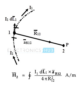
Consider a direct current is applied to a conductor. It produces a steady magnetic field around it. The Biot-Savart law is used to find the differential magnetic field intensity produced dH ̅ at point P due to a differential current element IdL.
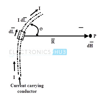
Consider the above figure in which the differential length is dL and the differential current element is IdL. The distance between the differential current element and point P is R and ɵ is the angle between differential current element and the line joining point P to the differential current element.
According to the Biot-Savart law, the magnetic field intensity produced at point P at distance R from a differential current element IdL is directly proportional to the multiplication of current I and differential length dL, sine of the angle between the element and the line joining point P and the element, and inversely proportional to the square of the distance R between the element and the point P.
Mathematically
dH ̅ α (I dL Sin ɵ)/ R2
dH ̅ = k (I dL Sin ɵ)/ R2
Where K is the proportionality constant and is equal to 1/4π
Thus,
dH ̅ = (I dL Sin ɵ)/ 4π R2 ……….. (1)
In vector form, Let dL = magnitude of vector length dL ̅ and
(aR) ̅ = unit vector in the direction from differential current element to P
According to the cross rule product,
dL ̅ × (aR) ̅ = dL |(aR) ̅ | Sin ɵ
= dL Sin ɵ since |(aR) ̅ | = 1
Substituting in the equation we get,
dH ̅ = (I dL ̅ ×(aR) ̅)/ 4π R2A/m ……………. (2)
But (aR) ̅ = R ̅/R
Therefore, dH ̅ = (I dL ̅ ×R ̅)/ 4π R3 A/m ……………….. (3)
To obtain the entire magnetic field intensity, the equation 2 has to be integrated as
H ̅ =∮(I dL ̅ ×(aR) ̅)/ 4π R2 A/m
By considering the closed path of the circuit as shown in figure, the field intensity between the two points is given as
Ampere’s Circuital Law
This law is analogous to the Gauss law in electrostatics. By using this law, complex problems are solved in magnetostatics. This law can be used to find the magnetic field intensity due to any current distributions.
According the Ampere circuital law, the line integral of magnetic field intensity H ̅ around a closed path is equal to the direct current enclosed by that path.
Mathematically,
∮H ̅.(dL) ̅=I
The above relation is called as an integral form of Ampere’s circuital law.
Where I is the current enclosed by the closed path.
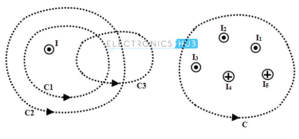
The concept of enclosed current is shown in below figures where the current I is enclosed by the closed paths C1 and C2. So along the either paths, the line integral of field intensity will give same result as I.
But the closed path C3 does not enclose any current and hence line integral of field intensity around that loop is zero.
In figure b, the closed path C is enclosed by several currents so the line integral of field intensity H around this closed path is equal to the algebraic sum of all the currents.
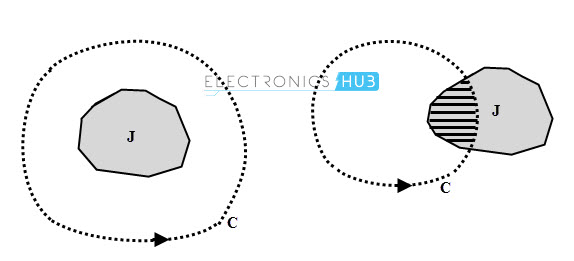
Now consider that the current is distributed continuously on an open surface, then the current distribution or current density J is the current per unit area. Therefore, the Ampere’s circuital law can be written as
Thus, the surface integral must be evaluated over the area of current carrying surface which is enclosed by the chosen closed path. In the below figure, the line integral of field intensity around the path C is equal to the entire current, whereas in case of second figure only the hatched area gives the current enclosed.
Therefore, it is necessary to know the nature of field variation before applying this law to a specific problem, so that a suitable closed path is chosen.
Magnetostatic Energy
Similar to a capacitor (which stores energy in the electric field), an inductor stores the energy in magnetic field. The energy stored by the inductor is given as
Wm = ½ LI2
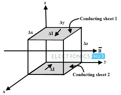
Consider the above figure, in which a magnetic filed B is exist in a differential volume. Then the inductance in a differential volume is given as
ΔL = ΔΦ / ΔI
= B ΔS / ΔI
Where ΔS = Differential surface area = Δx Δz
ΔL = B (Δx Δz) / ΔI
The differential current ΔI can be expressed in terms of the magnetic field intensity H as
ΔI = H Δy (since the current flow through the conducting sheets is in y direction)
Thus, the energy stored in the inductance of a differential volume is given as
Δwm = ½ ΔL ΔI2
Substituting ΔL and ΔI then
Δwm = ½ (B (µH Δx Δz) / H Δy)(H Δy)2
Δwm = ½ µH2 (Δx Δy Δz)
But the differential volume Δv = (Δx Δy Δz)
Δwm = ½ µH2 Δv
The magnetostatic energy density is obtained by
wm = lim(Δv→0)(Δwm/Δv)
Then wm = ½ µH2
The above equation can be written in different forms as
wm = ½ (µH) H = ½ BH2 and
wm = ½ B (B/µ) = ½ B2/µ
The energy in a magnetostatic field in a linear medium is given as
Wm = ∫wm
= ½ ∫µH2 dv.
Wm = ½ ∫B2 /µ dv.
Wm = ½ ∫BH dv
Magnetic Circuits
The magnetic circuits can be series, parallel or a combination of series and parallel. Some of the practical and common magnetic circuits are transformers, motors, toroid, generators, relays and magnetic recording devices.
Series Magnetic Circuit
Consider a simple magnetic circuit shown below that consist of uniform cross section area A, series magnetic flux path l, and a small air gap of length lg. Similar to the resistance, the opposition to the flux is called reluctance which is given as R in this magnetic circuit.
The equivalent electric circuit is also shown below. Since it is a series circuit, the same flux is flowing through two mediums, namely iron and air. Hence, the total reluctance offered against the magnetic fields will be sum of reluctances of air and iron.
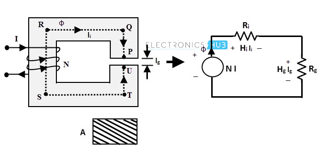
Since the cross section area is same, the flux density will be Φ/A and is constant in both iron and air paths. But the permeability of the medium is different, hence the magnetic field strength H will be different.
H required for iron, Hi = B / µoµi
H required for air. Hg = B / µo
According to the ampere circuital law, N*I = Hili + Hglg
= (B / µoµi) li + (B / µo) lg
= (Φ/ µoµi A) li + (Φ/ µoA) lg
N*I = ΦRi + ΦRg
Φ = N*I / (Ri + Rg)
From the above equation, it is expected that the reluctances are connected in series. So for a series magnetic circuit the total reluctance will be the sum of individual reluctances.
Points to ponder about the series magnetic circuit are the magnetic flux through all the parts of the circuit is same, equivalent reluctance is the sum of individual reluctances at different parts and the resultant mmf is the sum of mmf in each individual part.
Series-Parallel Magnetic Circuit
If a magnetic circuit consists of more than one path for the flux is known as a parallel magnetic circuit. In case of such magnetic circuit, different reluctances may be in parallel. Similarly, a combination of series and parallel circuits can be constructed. Consider the below figure which is a combination of both series and parallel magnetic circuits.
The terminology used for vertical links of the core is limbs of the magnetic circuit and that for horizontal links of the core is yoke of the magnetic circuit. From the following figure, PU, QT and RS are limbs and PQ, QR, UT and TS are yokes. In this, the total flux is divided into two components as Φ1 and Φ2.
The flux Φ1 completes its path through QTUP and the flux Φ2 through QRST. The relative values of Φ1 and Φ2 are decided by the reluctances of the respective paths.
The path TUPQ has same material and same cross sectional area, then the reluctance of this path is proportional to lTUPQ / A.
The central limb has the flux Φ1 that encounters two materials, namely iron (QM and WT) and small air gap (MW).
The reluctance of the air gap, Rg = lg / µoA.
The reluctance of the central limb of magnetic material is R1 = RQM+RWT.
And the portion of magnetic circuit that carries flux Φ2 has the reluctance R2 which is proportional to the lQRST / A.
Here, R2 = RQRST
The complete circuit showing the reluctances for two parallel magnetic paths is shown below.
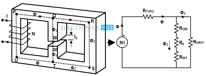
From the above circuit,
Total flux is sum of individual fluxes
Φ = Φ1 + Φ2
MMF balance in loop 1 is
NI = H1 + H1 * l1 + Hg * lg
= R Φ + (R1 + Rg) Φ1
MMF balance in loop 2 is
(R1 + Rg) Φ1 = R2 * Φ2
H1 * l1 + Hg * lg = H2 * l2
MMF balance in outer loop is
N*I = H1 + H2 * l2