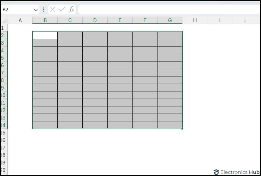
Ever struggle with your Excel spreadsheet, trying to keep track of rows and columns? Gridlines are here to help! These lines make it easier to navigate your data and format your worksheet. They’re usually there by default, but sometimes they vanish or you might want to tweak them for better visibility. Let’s see how to add gridlines in Excel, whether you’re on a Desktop (Windows or Mac) or using a Mobile device. Let’s dive in!
Outline
Toggle- What Are Gridlines In Excel?
- How To Insert Gridlines In Excel Desktop?
- How To View Gridlines In Excel Mobile?
- How To Insert Gridlines To Multiple Sheets At A Time?
- How To Put Gridlines To Specific Cells In Excel Sheet?
- How To Print An Excel Sheet With Gridlines?
- How To Remove Gridlines In Excel Sheets?
- FAQs:
- Conclusion
What Are Gridlines In Excel?
Gridlines in Excel are the faint, gray lines that outline cells on a worksheet. They make it easier to read and navigate through the data by visually organizing and separating cells. Gridlines form a grid-like pattern that divides the worksheet into rows and columns, running vertically and horizontally.
When you print a worksheet, gridlines don’t appear unless you set them to print. They are useful for designing or formatting a worksheet and providing a visual reference for aligning and positioning data, text, and objects within cells. Gridlines help maintain consistency and clarity in your Excel worksheet layout.
While gridlines are usually visible by default, they may be absent due to specific settings. In such cases, users can manually insert gridlines to improve the visual clarity of their worksheets.
How To Insert Gridlines In Excel Desktop?
Adding gridlines to your Excel worksheet can improve its readability and make it easier to work with your data. Excel offers easy ways to do it, allowing you to customize the appearance of your worksheet to suit your needs. Whether you’re a Windows user or a Mac user, the process is the same. Let’s explore how you can insert gridlines in Excel on your desktop.
Adding Gridlines Using View Tab
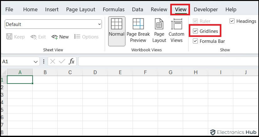
The View tab in Excel provides several options to customize the way your worksheet is displayed. One of these options is to show or hide gridlines. Here’s how you can add gridlines using the View tab:
- Open your Excel worksheet.
- Click on the View tab in the Excel ribbon at the top of the window.
- In the “Show” group on the View tab, check the box next to “Gridlines.”
Once you’ve checked the Gridlines box, you should see the gridlines appear on your worksheet
Adding Gridlines Using Page Layout Tab
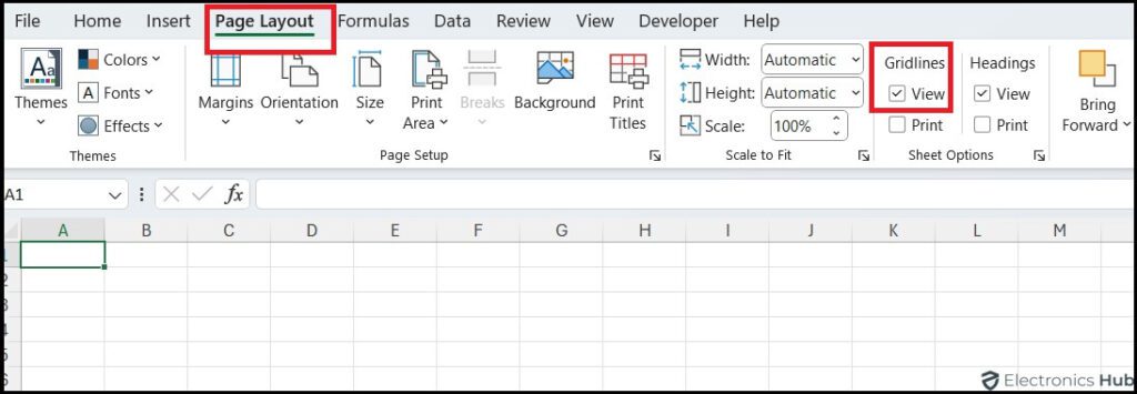
Alternatively, you can also add gridlines to your Excel worksheet using the Page Layout tab. Here’s how:
- Open Excel and the worksheet where you want to add gridlines.
- Click on the “Page Layout” tab in the Excel ribbon.
- In the “Sheet Options” group, find the “Gridlines” checkbox under “View.”
- Check the box to display gridlines on your worksheet.
How To View Gridlines In Excel Mobile?
You can also insert gridlines on your mobile device if they’re not already visible. Here’s how you can do it:
- Open the Excel Mobile app on your device.
- Locate and select the spreadsheet you want to view.
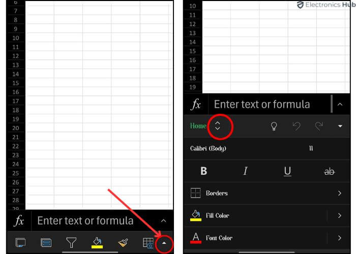
- Tap the upward arrow button at the bottom right corner of the screen.
- Next, tap the upward and downward arrow next to the “Home” tab.
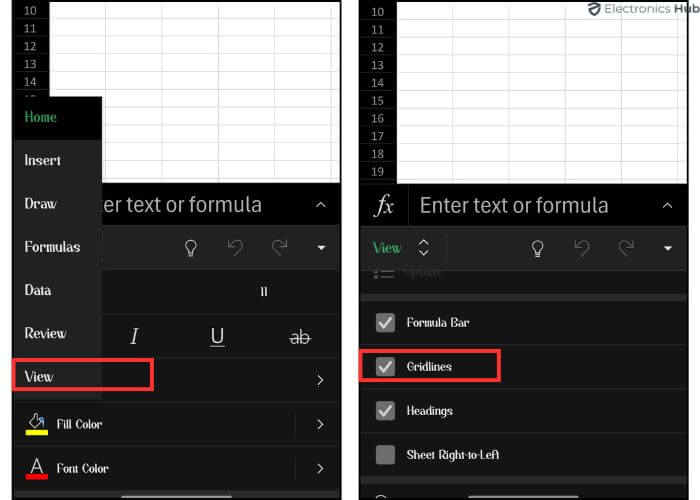
- From the menu that appears, select the “View” tab.
- Scroll down within the “View” tab to find the “Gridlines” option.
- Check the box next to “Gridlines” to enable them.
How To Insert Gridlines To Multiple Sheets At A Time?
Inserting gridlines into multiple sheets at once in Excel can save you time and effort, especially when working with large workbooks containing multiple sheets. Here’s how you can do it:
- Press and hold the Ctrl key (Command key on Mac).
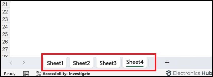
- Click on the sheet tabs at the bottom of the Excel window to select the sheets you want.
- Alternatively, right-click on any sheet tab and choose “Select All Sheets.” Then, deselect any sheets you don’t want to include.
- With the sheets selected, go to the “Page Layout” tab on the Excel ribbon.
- In the “Sheet Options” group, check the box next to “View” under “Gridlines.”
- Click on any sheet tab to see the changes. The gridlines should now be visible on all selected sheets.
How To Put Gridlines To Specific Cells In Excel Sheet?
Excel doesn’t allow you to add gridlines to specific cells within a worksheet. Gridlines are a global setting that applies to the entire sheet or workbook.
However, you can achieve a similar effect using cell borders. Here’s how:
- Choose the cells where you wish to simulate gridlines by clicking and dragging to highlight a range or by holding down the “Ctrl” key and clicking on individual cells.
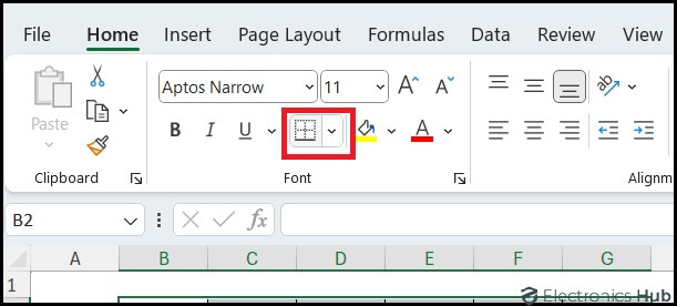
- Next, head to the Home tab on the ribbon.
- Find and click on the Borders dropdown menu within the Font section.
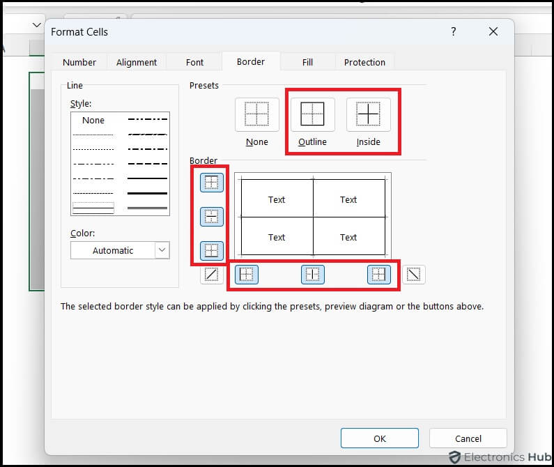
- Select “More Borders” from the dropdown menu. This will prompt you to the format cells window on the Border tab.
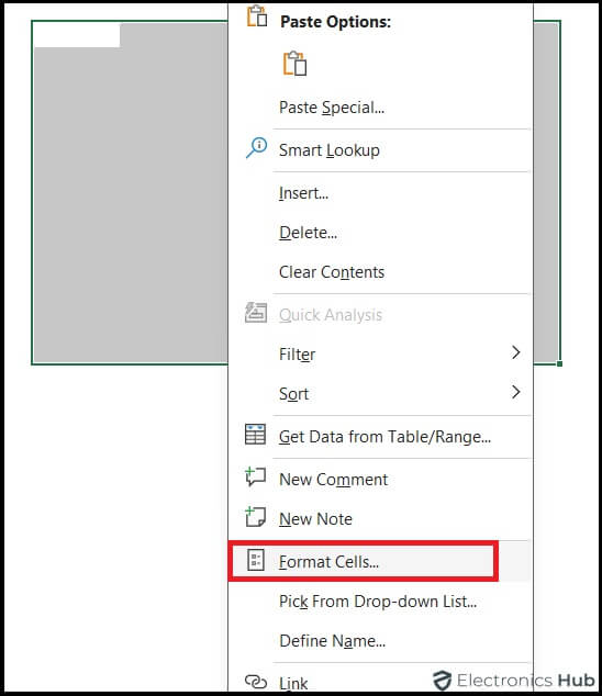
- Alternatively, you can also right-click on the selected area and choose the “Format Cells” option, then switch to the Border tab.
- To ensure borders are visible, ensure that the outline and inside options are selected in the presets section, and in the borders section, all options are selected as indicated below.
- You can also use this process to adjust the color of your borders to your preference.
- Once done, click “OK” to apply the changes.
Note: Keep in mind that gridlines and borders in Excel are not the same. Gridlines cannot be customized in the same manner as borders.
How To Print An Excel Sheet With Gridlines?
As we discussed earlier, when you print your worksheet from Excel, gridlines don’t appear by default. However, you can easily include them in your printed copy to enhance readability and maintain the structure of your data. Here’s how you do it:
- Open the worksheet you want to print with gridlines.
- Make sure gridlines are inserted into the worksheet before printing. If not, follow one of the methods we discussed earlier to insert them.
- Once gridlines are inserted, go to the “Page Layout” tab on the Excel ribbon.
- In the “Page Layout” tab, find the “Sheet Options” group.
- Look for the “Gridlines” section within the “Sheet Options” group.
- Check the box next to “Print” under the “Gridlines” section.
Once you’ve enabled gridlines, just go to the “File” tab, choose “Print,” then adjust your printer settings if needed. Your worksheet will now print with gridlines.
How To Remove Gridlines In Excel Sheets?
While gridlines can help organize data, there may be instances where you want to remove them for a cleaner appearance. Here’s how:
- Click on the “View” tab in the Excel ribbon at the top of the window.
- In the “Show” group on the View tab, uncheck the box next to “Gridlines.” This will remove the gridlines from your worksheet.
If you want to learn more about removing gridlines in Excel, refer to our comprehensive guide on how to remove gridlines in Excel.
FAQs:
To add gridlines to Excel’s Quick Access Toolbar, go to the View tab on the Excel ribbon. Find ‘Gridlines’ in the Show group. Right-click on ‘Gridlines,’ and choose ‘Add to Quick Access Toolbar’ from the menu. This puts the Gridlines button in the toolbar, so you can show or hide gridlines in your worksheets with a single click.
Gridlines might not show up in Excel for a few reasons. One common cause is that the “Gridlines” option might be turned off. To check, go to the “View” tab in Excel, and make sure “Gridlines” in the “Show” group is selected. If it’s already selected and gridlines still don’t show, they might blend with the background color. Change gridline color by going to “Page Layout,” then “Page Setup,” “Sheet,” and adjusting the color under “Gridlines.” If none of these work, there may be an issue with Excel’s settings or the worksheet itself.
To change the color of gridlines in Excel, follow these steps:
* Go to the “Page Layout” tab in the Excel ribbon.
* Click on the “Page Setup” group, then select “Print Titles”
* Locate the “Gridlines” section.
* Click on the dropdown menu next to “Color” to choose a new color for the gridlines.
* Click “OK” to apply the changes.
Yes, you can use the shortcut “Alt + W + VG” to quickly toggle gridlines on or off in Excel.
Yes, you can insert gridlines in Excel Online. The process is similar to the desktop version of Excel. Look for the “View” tab and toggle the “Gridlines” option to display them.
Conclusion
There you have it! With gridlines turned on, you can easily navigate through your spreadsheet and visually organize your data. Do follow the steps above to show or hide gridlines depending on your needs. Remember, gridlines by default won’t print on your worksheets, so you’ll need to enable that option in the Page Layout tab if you want them to appear in your printed copies. If this guide helped, feel free to leave a comment below!

