In the previous tutorials, we have seen the basics of Electric Charge and Coulomb’s Law. In this tutorial, we will continue exploring the concepts of electrostatics by understanding Electric Field.
We will try to get a picture of electric field, electric field lines and its properties, electric field due to different charge distributions (point charge, dipole, line of charge etc.).
Introduction
If you recall the previous topics on electric charge and Coulomb’s Law, we can say that Coulomb’s Law defines the electric force between two electric charges i.e. when an object of charge q1 is placed near another object of charge q2, then q1 experiences a force, which can be determined using the Coulomb’s Law.
An interesting question may arise as how the electric charge q1 “knows” the presence of charge q2 when separated by a distance and do not touch each other? How q2 can push (or pull) q1 by exerting the force?
The answer to all these questions is Electric Field. Similar to Gravity, the electric field is simply the presence of the charge which represents the “region of its influence”.
What is Electric Field?
Consider a point charge q1. If another charge q2 is brought near q1, then q2 experiences a force (we know this from Coulomb’s Law). What if q2 is moved around q1? Even then q2 experiences the force, as shown in the following image.
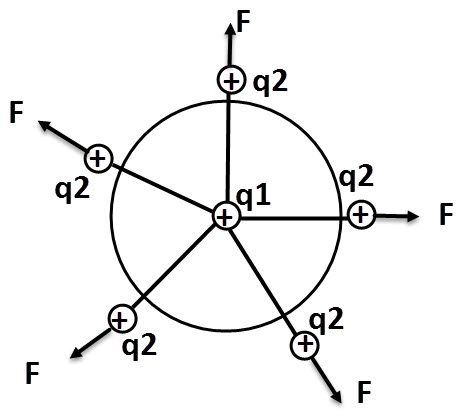
This implies that there is a region around the charge q1, where it exerts a force on any other charges (like q2 in this case). The region where a charge exerts a force on any other charge in that region is called Electric Field of that charge.
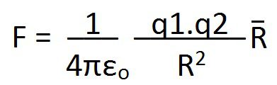
According to Coulomb’s Law, the force experienced by charge q2 due to charge q1 is given below:
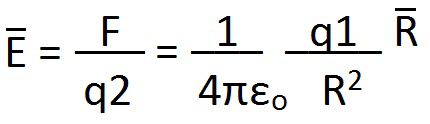
If we write the above equation as force per unit charge, then we get the following equation:
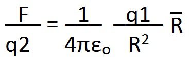
This is Electric Field (or electric field intensity) and is equal to force exerted per unit charge. It is a vector quantity denoted by . The direction of this vector is line joining q1 and q2.
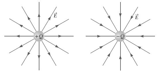
The electric field around a charged object is represented using imaginary lines of forces called Electric Field Lines. For a positive charge, these lines emanate radially outward from the charge. In contrast, for a negative charge, the lines are directed inwards, towards the charge.
Measuring E using a Test Charge
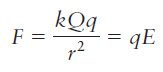
Consider a point charge whose electric field is E. Now, if we place a charge q (also called as the test charge) at a distance r from the point charge, it experiences an electric force as per the following equation.
![]()
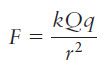
Using Coulomb’s Law, we can calculate the force exerted by the point charge Q on a test charge q as follows:
Using the above equation in the earlier equation we get:
Further, we can calculate E using the above equation as follows:
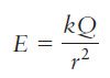
Units of E
As per the above discussion, electric field is defined as electric force per unit charge. Hence,
E = Force / unit charge = Newtons / Coulomb = N / C
Therefore, the units of E are N / C. It can also be measured in volts per meter (V / m).
Electric Field due to Different Charge Distributions
Now, let us see how we can determine the electric field due to different types of charge distributions. For this tutorial, we will four types of charge distributions: Point Charge, Electric Dipole, Line of Charge and Charged Disk.
Point Charge
This is very simple and we have already seen the equation for a point charge. But let us find the electric field due to a point charge. Assume a point charge q. Let us place another charge qo (a test charge) at a distance r from the point charge.
From Coulomb’s Law, the electric force acting on the test charge is given by the following equation:
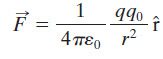
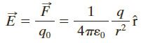
If the point charge q is positive, then the direction of F is away from the charge and if q is negative, the direction of F is toward the point charge. Keeping this in mind, we can now calculate the E as follows:
Electric Dipole
The following image shows a setup of two charges that are equal in magnitude and are opposite in sign. This configuration is often called as Electric Dipole.
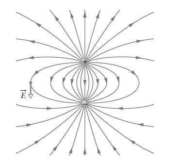
Let us now find the E due to an electric dipole. The following image shows two charged particles of same magnitude q but of opposite sign. They are separated by a distance d. the axis through the charged particles is called Dipole Axis and we will find the E at point P, which is at a distance z from the mid-point of the dipole axis.
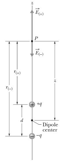
Using superposition principle for electric fields, the magnitude of E at P is given by the following equation:
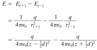
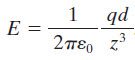
Using a little algebra in the above equation and also assuming that distance z is much greater than d (z >> d), we get the following equation.
Line of Charge
The charge distribution discussed so far are considered to b discrete. But some charge distributions consist of many tightly placed point charges (in the number of millions or billions) that are spread along a line or over a surface or within a volume.
Such distributions are considered to be continuous and, in this case, it is easy to express the charge of the object as charge density instead of total charge. In case of a line of charges, we use the linear charge density, represented by λ (units C / m).
Now consider an insulator ring of radius R. Around its circumference, there is uniform positive charge density λ. We will now calculate E at a point P which is at a distance z from the plane of the ring along its central axis.
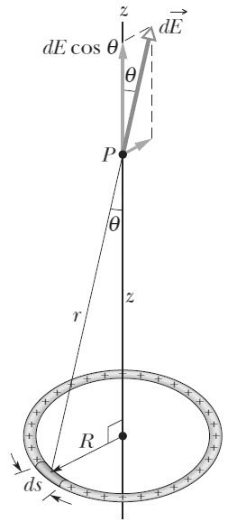
We cannot directly calculate E as the ring is not a point charge. So, we divide the ring into several differential elements of charge which are identical to a point charge.
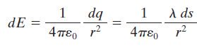
We know that λ is the charge per unit length let us assume ds to be length of the differential element. Then the magnitude of charge of this differential element is:
dq = λ ds
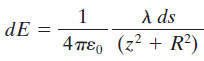
Since the charge is differential, the E at point P is also differential and is given by the following equation.
Using a little trigonometry, we can write the above equation as follows:
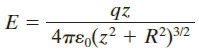
Now, after adding the parallel component, integrating for the entire circumference and substituting for λ, we get E as:
Charged Disk
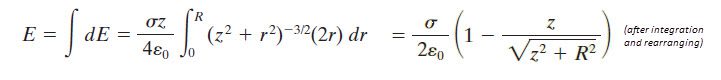
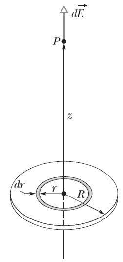
Consider an insulated circular disk of radius R with a positive surface charge density of σ (charge per unit area). We will now calculate E at a point P, which is at a distance z from the disk along its central axis.
Similar to the previous line of charge calculation, we will divide the disk into concentric rings and calculate the E by integrating. Let one of concentric rings have a radius of r and radial width of dr.
If σ is the charge per unit area and dA is the differential area of the ring, then the charge of the ring is
dq = σ dA = σ (2πr dr)
From the previous ring of charge calculation, dE due to flat ring is given by
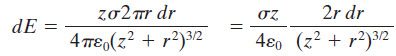
Integrating this over the surface of the disk and rearranging, we get E of a charged disk as follows: