A Butterworth Filter is a type of Active Filter, where the frequency response of the across its pass band is relatively flat. Because of this frequenct response, Butterworth Filters are also known as Maximally Flat Filters or Flat-Flat Filters.
Using Butterworth Filter technique, you can design all types of filters i.e. High Pass, Low Pass, Band Pass etc. In this tutorial we will concentrate on Low Pass Filter Design using Butterworth Filter Technique.
For more information on typical Low Pass Filters, whether Active or Passive, read these tutorials: “Passive Low Pass RC Filters” and “Active Low Pass Filters“.
Introduction
There are mainly three considerations in designing a filter circuit they are
- The response of the pass band must be maximum flatness.
- There must be a slow transition from pass band to the stop band.
- The ability of the filter to pass signals without any distortions within the pass band.
These distortions are generally caused by the phase shifts of the waveforms. In addition to these three the rising and falling time parameters also play an important role. By taking these considerations for each consideration one type of filter is designed.
For maximum flat response the Butterworth filter is designed. For slow transition from pass band to stop band the Chebyshev filter is designed and for maximum flat time delay Bessel filter is designed.
Butterworth Filter
At the expense of steepness in transition medium from pass band to stop band this Butterworth filter will provide a flat response in the output signal. So, it is also referred as a maximally flat magnitude filter.
The rate of falloff response of the filter is determined by the number of poles taken in the circuit. The pole number will depend on the number of the reactive elements in the circuit that is the number of inductors or capacitors used in the circuits.
The amplitude response of nth order Butterworth filter is given as follows:
Vout / Vin = 1 / √{1 + (f / fc)2n}
Where ‘n’ is the number of poles in the circuit. As the value of the ‘n’ increases the flatness of the filter response also increases.
‘f’ = operating frequency of the circuit and ‘fc‘ = centre frequency or cut off frequency of the circuit.
These filters have pre-determined considerations whose applications are mainly at active RC circuits at higher frequencies. Even though it does not provide the sharp cut-off response it is often considered as the all-round filter which is used in many applications.
Butterworth Approximations
As we know that to meet the considerations of the filter responses and to have approximations near to ideal filter we need to have higher order filters. This will increase the complexity.
We know the output frequency response and phase response of low pass and high pass circuits also. The ideal filter characteristics are maximum flatness, maximum pass band gain and maximum stop band attenuation.
To design a filter, proper transfer function is required. In order to satisfy these transfer function mathematical derivations are made in analogue filter design with many approximation functions.
In such designs Butterworth filter is one of the filter types. Low pass Butterworth design considerations are mainly used for many functions. Later we will discuss about the normalized low pass Butterworth filter polynomials.
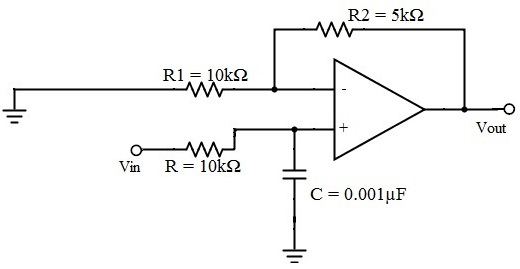
First Order Low Pass Butterworth filter
The below circuit shows the low pass Butterworth filter.
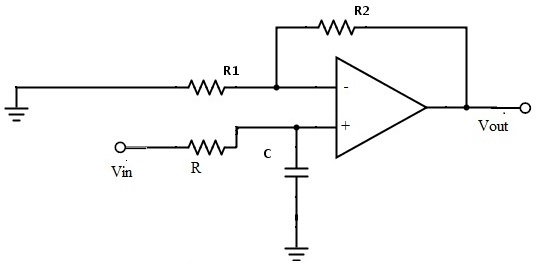
The required pass band gain of the Butterworth filter will mainly depends on the resistor values of ‘R1’ and ‘Rf’ and the cut off frequency of the filter will depend on R and C elements in the above circuit.
The gain of the filter is given as A_max=1+R1/Rf
The impedance of the capacitor ‘C’ is given by the -jXC and the voltage across the capacitor is given as,
Vc = – jXC / (R – jXC) * Vin.
Where XC = 1 / (2πfc), capacitive Reactance.
The transfer function of the filter in polar form is given as
H(jω) = |Vout/Vin| ∟ø
Where gain of the filter Vout / Vin = Amax / √{1 + (f/fH)²}
And phase angle Ø = – tan-1 ( f/fH )
At lower frequencies means when the operating frequency is lower than the cut-off frequency, the pass band gain is equal to maximum gain.
Vout / Vin = Amax i.e. constant.
At higher frequencies means when the operating frequency is higher than the cut-off frequency, then the gain is less than the maximum gain.
Vout / Vin < Amax
When operating frequency is equal to the cut-off frequency the transfer function is equal to Amax /√2 . The rate of decrease in the gain is 20dB/decade or 6dB/octave and can be represented in the response slope as -20dB/decade.
Second Order Low Pass Butterworth Filter
An additional RC network connected to the first order Butterworth filter gives us a second order low pass filter. This second order low pass filter has an advantage that the gain rolls-off very fast after the cut-off frequency, in the stop band.
In this second order filter, the cut-off frequency value depends on the resistor and capacitor values of two RC sections. The cut-off frequency is calculated using the below formula.
fc = 1 / (2π√R2C2)
The gain rolls off at a rate of 40dB/decade and this response is shown in slope -40dB/decade. The transfer function of the filter can be given as
Vout / Vin = Amax / √{1 + (f/fc)4}
The standard form of transfer function of the second order filter is given as
Vout / Vin = Amax /s2 + 2εωns + ωn2
Where ωn = natural frequency of oscillations = 1/R2C2
ε = Damping factor = (3 – Amax ) / 2
For second order Butterworth filter, the middle term required is sqrt(2) = 1.414, from the normalized Butterworth polynomial is
3 – Amax = √2 = 1.414
In order to have secured output filter response, it is necessary that the gain Amax is 1.586.
Higher order Butterworth filters are obtained by cascading first and second order Butterworth filters. This can be shown as follows:
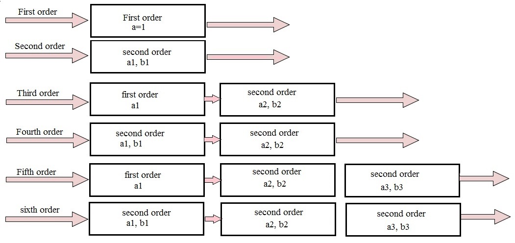 Where an and bn are pre-determined filter coefficients and these are used to generate the required transfer functions.
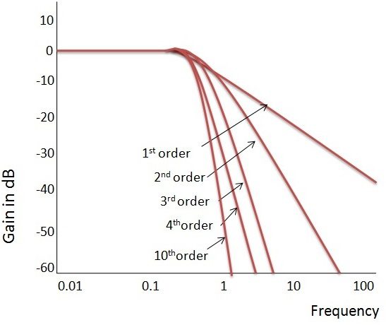
Ideal Frequency Response of the Butterworth Filter
The flatness of the output response increases as the order of the filter increases. The gain and normalized response of the Butterworth filter for different orders are given below.
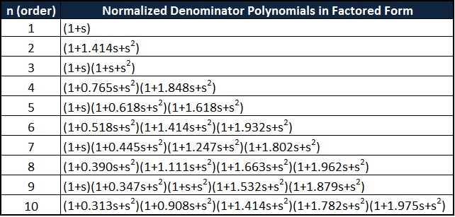
Normalized Low Pass Butterworth Filter polynomials
Normalization is a process in which voltage, current or impedance is divided by the quantity of the same unit of measure. This process is used to make a dimensionless range or level of particular value.
The denominator polynomial of the filter transfer function gives us the Butterworth polynomial. If we consider the s-plane on a circle with equal radius whose centre is at origin, then all the poles of the Butterworth filter are located in the left half of that s-plane.
For any order filter the co-efficient of the highest power of ‘s’ should be always 1 and for any order filter the constant term is always 1. For even order filters all the polynomial factors are quadratic in nature. For odd order filters all the polynomials are quadratic except 1st order, for 1st order filter the polynomial is 1+s.
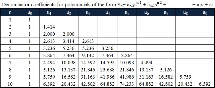
Butterworth polynomials in coefficients form is tabulated as given below.
The transfer function of the nth order Butterworth filter is given as follows
H(jω) = 1/√{1 + ε² (ω/ωc)2n}
Where n is the order of the filter
ω is the radian frequency and it is equal to 2πf
And ε is the maximum pass band gain, Amax
Butterworth Low Pass Filter Example
Let us consider the Butterworth low pass filter with cut-off frequency 15.9 kHz and with the pass band gain 1.5 and capacitor C = 0.001µF.
fc = 1/2πRC
15.9 * 10³ = 1 / {2πR1 * 0.001 * 10-6}
R = 10kΩ
Amax = 1.5 and assume R1 as 10 kΩ
Amax = 1 + {Rf / R1}
Rf = 5 kΩ
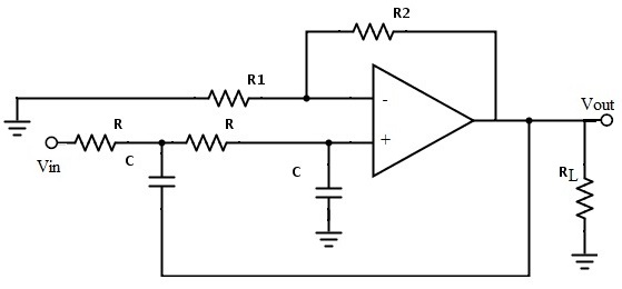
Third-order Butterworth Low Pass Filter
The cascade connection of 1st order and 2nd order Butterworth filters gives the third order Butterworth filter. Third order Butterworth filter circuit is shown below.
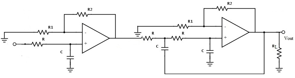
For third order low pass filter the polynomial from the given normalized low pass Butterworth polynomials is (1+s) (1+s+s²). This filter contains three unknown coefficients and they are a0 a1 a2.
The coefficient values for these are a0 = 1, a1 = 2 and a2 = 2. The flatness of the curve increases for this third order Butterworth filter as compared with the first order filter.
Applications
- Due to its maximum flat pass band nature it is used as anti-aliasing filter in data converter applications.
- It has applications in radars such as in designing the display of radar target track.
- In high quality audio applications these are used.
- These are used in digital filters for motion analysis.