The electromagnetism is a branch of physics that deals with electric and magnetic fields and their interaction with substance or matter on a microscopic level. The various domains in the electromagnetism are electrostatics, magnetostatics, electrokinetics and electrodynamics.
During the study in practical applications as well as for macroscopic phenomena, these domains are very useful. Similar to the gravitational force, electromagnetic forces are also long range and directly observable.
The electromagnetism phenomena involve in dealing with electromagnetic force which includes both electric charge and magnetism whether in motion or rest. Let us study this phenomenon of interaction of electric charges at rest called as electrostatics.
What Is Electrostatics?
Electrostatics is one of the fundamental subjects in potential theory as it is the origin for most of the equations and fundamental concepts used in electromagnetic theory. A branch of electromagnetism, which deals with the interaction of electric charges when all the charges are stationary is called as electrostatics.
The theory involved in electrostatics is, if an object surface contact with other surfaces, a charge is built up on its surface. This charge can be positive or negative and unlike charges attract each other, whereas like charges repel each other.
These electric charges of same or opposite polarities produce an electric field. A typical example is that the field produced in cathode-ray tube (CRO).
During the design of suitable equipments in case of electric power transmission, lighting protection, X-ray machines, a knowledge of electrostatics is required. Also in solid state electronic devices like transistors, the electron motion is controlled by electrostatic fields.
The various input/output devices like LCDs, capacitance keypads. Touchpads, electrostatic printers, CRO are the typical examples which works based on electrostatics. Therefore, electrostatics exist in diverse areas of application in our daily lives.
Electric Charge
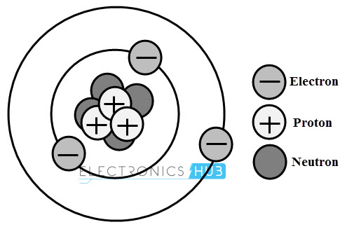
The charge is a characteristic property of certain elementary particles. In all substances, the charges are building blocks of an atom. The major kinds of charges include protons and electrons. The charge on the electron is negative, which revolves around the nucleus.
And the charge on the proton is positive which is located at the center of the atom i.e., nucleus. So the nucleus contains the positively charged proton and neutrons, which are electrically neutral as shown in below figure.
Generally, the positive charges of the protons are equal to the total negative charges of electrons so that the atoms of a body are electrically neutral. This neutral condition of some of the atoms of a body is disturbed when the body is charged either by subtracting or adding one or more electrons.
Then, the atom is said to negatively ionized if there is excess of electrons and positively ionized if there is a deficiency of electrons. Two particles with charges of same polarities repel each other and with same polarity attract each other.
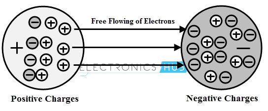
A static electricity is generated by the stationary charges. When a force or pressure applied to a material causes electrons to be removed from their atoms. This movement of electrons from one atom to the other is called as the electric current.
Substances having no freely movable charges in their structures called as insulators or dielectrics. Substances having elemental electric charges which are free to move inside of them are as called conductors. And a type of substances in which there are only a small number of free movable charges in their structures called as semiconductors.
Coulomb’s law
A French colonel, Charles Augustin de Coulomb was experimentally formulated a force that exists between the two charged bodies in 1785. He determined a direct relationship between the two point charges which are separated by a small distance.
So this law gives the electrostatic interaction between the electrically charged particles. This interaction is a non-contact force acts over some distance of separation.
This force may be repulsive or attractive depends on whether the charges on the bodies are opposite or same polarity and it is a vector quantity that has magnitude as well as direction.
Coulomb’s law states that the magnitude of the electrostatic force that exist between the two point charges is directly proportional to the scalar product of the magnitudes of point charges and inversely proportional to the square of the distance between the point charges.
Also, the electrostatic force is in the direction of the straight line joining the two point charges. This force is repulsive, if the two point charges are of the same sign and the force is attractive if they are of opposite sign.
Two conditions must be fulfilled for the validation of coulomb’s law; one is, the charges must be point charges and the other one is the charges must be stationary with respect to each other.
If the Q1 and Q1 are the two point electric charges at rest and are separated by a distance r then the force exerted on each other given as
F = K (Q1 × Q2)/r2
Where F = force in newtons
Q = charge in coulombs
r = distance in meters and
K is the constant which has the value
K = 1/ 4 π єo
єo is the permittivity of free space and its measured value is
єo = 8.8541 × 10⁻¹² C2/Nm2
Thus, K = 1/ 4 π єo = 8.987 × 10⁹ Nm2 C-2
But for most numerical applications, this value is considered as 9 × 10⁹ Nm2 C-2
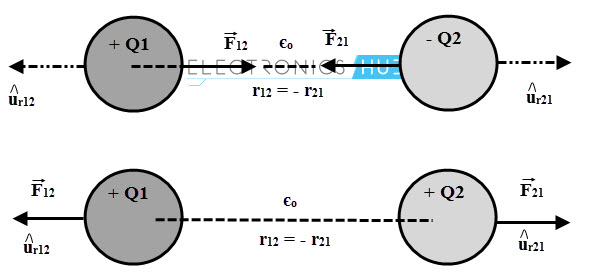
The above force equation only gives the magnitude of the force between the two points, but does not give any indication of direction. So further this equation can rewrite in a form involving vectors. The above figure shows the two point charges separated by the unit vectors. Then the equation of the forces F12 and F21 are
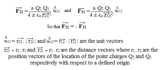
From the above equations we can say that, the force on Q1 due to Q2, F12 is equal and opposite to the force on Q2 due to Q1, F21.
Types of Electric Charge Distributions
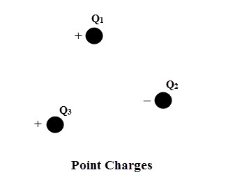
In the above the charge distribution is explained by considering the point charges. In addition, there is possibility to distribute the charge continuously along line, in a volume or on surface. Therefore, there are four types of charge distributions namely
- Point charge
- Line charge
- Surface charge
- Volume charge
Point Charge
Compared with region surrounded by a surface carrying a charge, the dimensions of that surface are very small, then that charge is treated as point charge. The point charge can be negative or positive. And it has a position but do not have dimensions.
 Line Charge
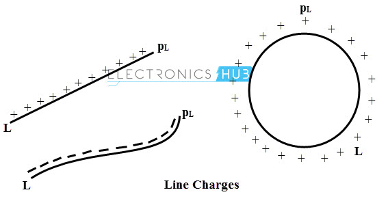
A charge possibly spread all along the line whether infinitely or finitely. A charge that uniformly distributed all along the line is called as line charge as shown in figure. The charge density of a line charge is defined as the charge per unit length and denoted as pL.
It is measured in coulomb per meter and is constant all along the length of the line charge. The examples of the line charge are a charged loop of a circular conductor and sharp beam in a CRO.
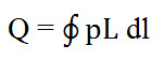
The total charge for the entire length L is obtained by applying line integral to the charge dQ (is equal to the pL) on dl as
Surface Charge
A surface charge is also called as sheet of charge in which the charge is uniformly distributed over a two dimensional surface. The area of the two dimensional surface is in square meters. The surface charge density is defined as the charge per unit surface area and is denoted as pS.
It is measured in coulomb per meter square and it is constant over the surface carrying the charge. The example of the surface charge distribution is the plate of a charged parallel plate capacitor.
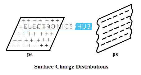
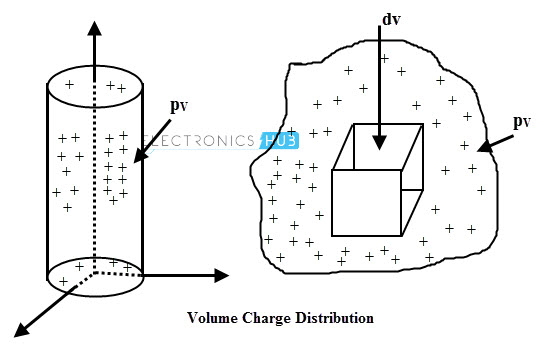
In surface charge distribution, the total charge distribution is determined by considering the charge dQ on elementary surface area ds over that surface. Thus, it considers the surface integral rather than normal integral. Mathematically
The distribution of the charge is considered as an infinite sheet of charge if the dimensions of the surface is charge is very large compared to the distance at which the effects of charge to be considered.
Volume Charge
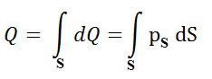
A volume charge is the charge which is distributed uniformly in a given volume. The volume charge density is defined as the charge per unit volume and is denoted as pV. It is measured in coulomb per meter cube. The example of this volume charge is the charged cloud.
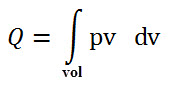
The total charge within a given volume is obtained by integrating dQ by a differential volume dv. This integral is called as volume integral and is given as
Electrostatic Field
Once the charge distribution of a particle is known, we can determine the electric field of that particle. As we know that substances constitute the point charges (electrons and protons) which results field from each of these point charges.
Suppose if a particle bearing a unit positive charge is placed at a specified point, then it experience a force which is called electric force F. the region in which this force exist is called as the region of electric field.
This is defined as the force per unit charge exerted on a tiny positive charge placed at that point and it is a vector quantity with a unit of Newton/coulomb.
The electrostatic field E is given as
E = F/q or F = Eq
Where F is the electrostatic force and q is the net electric test charge.
The above equation states that regardless of a second charge on the space surrounded by the net charge, it produces an electric field around that space. Consider that if the two point charges are exist in the region as shown in the above figure. Then the electric field intensity by considering Q2 as one coulomb is given as
E = (Q1/ (4 π єor212)) × r1
Where r12 is the distance between Q1 and Q2 and r1 is the unit vector in the direction of line joining Q1 with Q2.
And also F12 = Q2 E
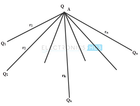
Consider that the above figure in which the region consists of n two point charges, then the electric field intensity at point A is given as
EA = Σk =1n (Qk / (4 π єor2k)) × rk1
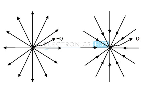
For a better visualization, the electric field is expressed in terms of lines of force or electric flux. Lines of force are continuous imaginary paths whose direction is along with the direction of vector E. Lines of force for positive and negative point charges are shown in below figure.
The lines of force for a positive charge are outward and in case of negative charge the lines of force are inward as shown in figure. So the space around this charge is filled with these lines of force and this charge in the field would experience a force whose direction is in the direction of lines of force.
The number of lines of force whether from positive or negative charges are depending on the magnitude of the particular charge. And the stronger will be the electric filed in a given region when lines are together closer.
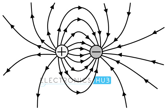
The lines of force or electric fields for two opposite and similar charges are shown in below figure. In case of two opposite charges, the lines of force are originated from the positive charge and terminate at negative charge. In case of two similar charges, at the neutral point the resultant field from two charges is zero as shown in figure.
The number of lines passing through a given surface is called as electric flux. For a closed surface the flux is negative if the lines of force point inward and positive if they point outward.

Gauss Law
Gauss law is one of the fundamental and general laws of electromagnetism that can be applied at to any closed surface called as Gaussian surfaces. A German physicist and mathematician Karl Friedrich Gauss published this theorem or law in 1867.
This law gives a relation between electric field intensity over a surface and a net charge enclosed by that surface. The Gaussian surfaces are the closed surfaces in which the electric field is either zero or constant. In most of the cases the electric field will be either tangential or normal to the Gaussian surfaces.
This law is applied to calculate the electric field intensity of Gaussian surfaces. Depends on the suitability, this law can be stated in two different ways namely integral and differential form.
Gauss law states that electric flux through a closed surface is proportional to the total charge enclosed by that surface. Mathematically
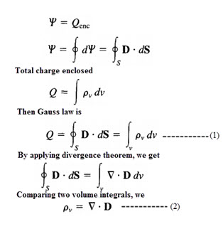
The above two equations are stating Gauss law in two different ways, i.e., integral form and differential or point form. In the above equations D is the electric flux density, pv is the volume charge density and integration symbol indicates the closed surface integral.
If the Gaussian surface constitutes more than one charge distribution, then the net charge is the algebraic addition of all the individual charges.
The Gauss theorem can be used to determine electric field intensity E, and electric flux density D for symmetrical charge distributions like infinite line charge, point charge, spherical distribution of charge and infinite sheet of charge. This law cannot be used if the charge distribution is not symmetric.
Electrostatic Potential
Suppose if a body is moved from one point to the other by a force, then the work is done by the body or on the body. In case of frictionless motion, the work done represents energy is not a dissipated one, but must be stored as either kinetic energy or potential energy.
So if a charge is moved in an electric field, there is no friction and hence no energy is dissipated. In this field, the zero or reference point is at the boundary of the region of the field so usually this point is taken as infinity.
The potential at a point in an electrostatic field is defined as the work done to bring a unit positive charge from infinity to point P.
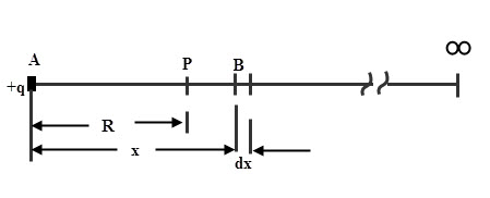
Consider the below figure, in which we determine the potential at point P. Let the charge q is responsible to produce the field in a given region which is placed at distance R from point P. Let B be a point which is located at the distance x from q. Then work done in moving a unit charge by an infinitesimal distance dx is
dw = – F dx
The negative sign represents the work done against the force and the force on a unit charge at point B is given as
F = q / 4πєx2
This force is constant for distance dx. Thus the work done to bring the a unit charge to point P from infinity is
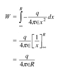
Hence the potential at the point P is,
V = q/ 4πєR
This potential has only magnitude and no direction, hence it is a scalar quantity. Thus the potential at a point is independent of the path followed. The potential which is caused from a positive charge is positive and the potential caused from negative charge is negative.
Similar to the potential, potential difference is the work done to bring a unit positive charge from one point to another.
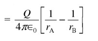
The potential difference between points A and B which are laid on the same line with a force, VAB is
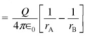
The potential difference in moving a unit charge from point B to A (two points are doesn’t laid on same path) , VAB is