Waves are omnipresent in nature that transfers the energy or information from source to destination. The wave is a function of both space and time. An exotic kind of wave is electromagnetic wave which existence is stated by the professor Heinrich Hertz but earlier Maxwell himself predicted the existence of electromagnetic waves.
These waves can travel through a vacuum or no medium. These are different from mechanical waves like sound waves which can travel or transport their energy through a medium of material.
So, unlike the mechanical waves, electromagnetic waves can travel through the vacuum. The typical examples of the EM waves are visible light waves, radio waves, radar beams and TV signals. The electromagnetic waves subject is a composite phenomenon of electric and magnetic fields.
Uniform Plane Wave and Wave Equation
The basic understanding of the electromagnetic wave propagation in medium is provided by the basic concept of uniform plane wave. The uniform plane wave is a fundamental concept in electro magnetics and it is the simplest solution to the Maxwell’s equation for time varying fields in an unbound, homogeneous medium.
Although such medium as unbound, homogeneous does not exists in practice, the fundamental concept of uniform plane wave is very useful for the knowledge of electromagnetic waves. Also, uniform plane wave solution is quite useful and adequate in many problems practically.
In some cases where the media have physical dimensions much larger than the wavelength, then the solution closely approximates the uniform wave solution.
Consider a homogeneous, isotropic, unbounded medium without consisting of any electric or magnetic source. In such case, the medium permeability µ and permittivity є are constant over the entire medium. Since the medium is of source free and hence there are no free charges in the medium. The Maxwell’s equations are given as
∇ .D‾= 0
∇ . B̅ = 0
∇ × E̅ = − ∂B̅/ ∂t
∇ × H̅ = J̅ + ∂D̅/ ∂t
From constitutive relations,
B̅ = µ H̅
D̅ = є E̅
J̅ = σ E̅
The permeability µ and permittivity є are constant as a function of time and space due the homogeneous and non-time varying medium. Thus the Maxwell’s equations become,
∇ . B ̅ = ∇. (µ H ̅) = µ ∇. H ̅ = 0
∇. H ̅ = 0 ……….(1)
∇ . D ̅ = ∇. (є E ̅) = є ∇. E ̅ = 0
∇. E ̅ = 0 ……….(2)
∇ × E ̅ = − ∂ (µ H) / ∂t
∇ × E ̅ = − µ ∂ H ̅ / ∂t ………. (3)
∇ × H ̅ = ∂ (є E ̅ ) / ∂t
∇ × H ̅ = σ E ̅ + є ∂ E ̅ / ∂t ………. (4)
In above, ∇ indicates the differentiation with respect to space while ∂ / ∂t indicate differentiation with respect to time. From the above 3 and 4 equations, we can say that the time derivative of the magnetic field is related to the space derivative of the electric field and also, the time derivative of the electric field is related to the space derivative of the electric field.
Thus, from these two equations it is to be noted that a time varying magnetic field cannot exist without corresponding electric and magnetic field. Therefore, both magnetic and electric fields must be co-exist to produce the time varying fields.
For such time varying fields, we cannot get only magnetic or only electric time varying fields. But in case of time invariant fields like electrostatic and magnetostatic fields can exist without each other.
Taking the curl of equation 3 and 4, we get
∇ × ∇ × E ̅ = − µ ∇ × ∂ H ̅ / ∂t
∇ × ∇ × H ̅ = ∇ × (σ E ̅ ) + ∇ (є ∂ E ̅ / ∂t)
Both ∇ and ∂ / ∂t are independent of each other hence the operators can be interchanged as
∇ × ∇ ×E ̅ = − µ × ∂ (∇ ×H ̅) / ∂t
∇ × ∇ × H ̅ = σ (∇ × E ̅ ) + є × ∂ (∇ × E ̅) / ∂t
Substituting the (∇ × H) and (∇ × E) values from 3 and 4 equations, we get
∇ × ∇ × E ̅ = − µ × ∂ / ∂t (σ E ̅ + є ∂ E ̅ / ∂t)
∇ × ∇ × E ̅ = − µ σ × ∂ E ̅/ ∂t − µ є (∂2 E ̅ / ∂t2)
Similarly
∇ × ∇ × H ̅ = σ (− µ ∂ H ̅ / ∂t) + є × ∂ / ∂t (− µ ∂ H ̅ / ∂t)
= − µ σ (∂ H ̅ / ∂t) − µ є (∂2 H ̅ / ∂t2)
Using the vector identity ∇ × ∇ × A = ∇ (∇. A) − ∇2 A, where A is the any arbitrary vector, then the above equations can be written as
∇ (∇.E ̅) − ∇2E ̅ = − µ × ∂ / ∂t (σ E ̅ + є ∂ E ̅ / ∂t)
∇ (∇.H ̅) − ∇2 H ̅ = − µ σ × ∂ E ̅/ ∂t − µ є (∂2 E ̅ / ∂t2)
But equations 1 and 2, (∇.E ̅) = 0 and (∇.H ̅) = 0 then
− ∇2 E ̅ = − µ σ × ∂ E ̅/ ∂t − µ є (∂2 E ̅ / ∂t2)
∇2 E ̅ = µ σ × ∂ E ̅/ ∂t + µ є (∂2 E ̅ / ∂t2) ……(5)
This is the wave equation for the electric field E ̅ for a medium. And similarly
−∇2 H ̅ = − µ σ (∂ H ̅ / ∂t) − µ є (∂2 H ̅ / ∂t2)
∇2 H ̅ = µ σ (∂ H ̅ / ∂t) + µ є (∂2 H ̅ / ∂t2) ……(6)
This is the wave equation for the magnetic field for a medium.
The above 5 and 6 equations are the wave equations and their solutions represent the wave phenomenon in three dimensional space. Finally, we conclude that for the existence of time varying fields in a homogeneous, unbounded medium, they have to exist in the form of a wave.
In addition, there must exist both electric and magnetic fields together. That’s how this phenomenon is called as an electromagnetic wave.
But for free space, J = 0, σ = 0, є = єo and µ = µo. Substituting these values in 5 and 6 equations we get
∇2 E ̅ = µo єo (∂2 E ̅ / ∂t2)
∇2 H ̅ = µo єo (∂2 H ̅ / ∂t2)
EM waves are travelling in the direction of Z plane, hence both vectors E ̅ and H ̅ are independent of x and y. Thus the vectors E ̅ and H ̅ are the function of z and t. Therefore, the above equations becomes
∂2 E ̅ / ∂z2= µo єo (∂2 E ̅ / ∂t2)
By rearranging the terms, we get
∂2 E ̅ / ∂t2= (1/µo єo) (∂2E ̅ / ∂z2)
According to the results in physics,
Velocity of the light v = (1/√(µo єo)) = 3 × 10⁸ m/s
v2 = (1/µ є)
Substituting in the above equation we get
∂2E ̅ / ∂t2= v2 (∂2 E ̅ / ∂z2)
Similarly ∂2H ̅ = v2 (∂2H ̅ / ∂t2)
Plane wave propagation
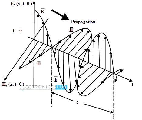
Electromagnetic waves in a medium are characterized by the electrical parameters like permeability, permittivity and conductivity. EM waves are associated with both electrical and magnetic fields which are perpendicular to each other as well as perpendicular to the direction of propagation.
Generally, the direction of propagation is to be taken along the Z axis. The velocity of propagation for all EM waves in a free space is equal to the velocity of the light i.e., 3 × 10⁸ m/s. The direction of the propagation is normal to the plane formed by the magnetic and electric field vectors.
And the phase of these fields is independent of x and y axes thereby no phase variation exist over the planar surfaces orthogonal to the direction of the propagation.
The waves that are uniform in magnitude and direction in the planes of a stated orientation are called as plane waves. The magnitudes of EM wave fields (electric and magnetic field) are constant in the xy – plane and the surface of constant phase forms a plane parallel to the xy-plane and hence these waves are termed as plane waves.
According to the Maxwell’s curl equations, the oscillating electrical field produces a magnetic flux which further oscillates in order to create the electric field. This interaction between these two fields cause to store the energy, thereby it carries the power.
The important properties of the waves are amplitude, phase or frequency, which allows the waves to carry the information from source to destination.
In particular, the uniform plane waves are EM waves which electric field is the function of x and time t and independent of y and z axes.
These waves are basically TEM waves (Transverse EM waves) in which the E and H fields always have constant magnitudes and are in time phase. The power transmitted by the E and H fields is in the direction of propagation.
EM Wave Polarization
It is important to know that the direction of the electric field vector changes with time for a uniform plane wave which decides the polarization of the wave. This is because some applications can only receive or transmit one type of polarized EM waves and the best example is different antennas in RF applications is designed for one type of polarized wave.
In a plane EM wave, the electric field oscillates in the x-z plane while the magnetic field oscillates in the y-z plane. Hence, it corresponds to a polarized wave. The plane in which the electric field oscillates is defined as the plane of polarization.
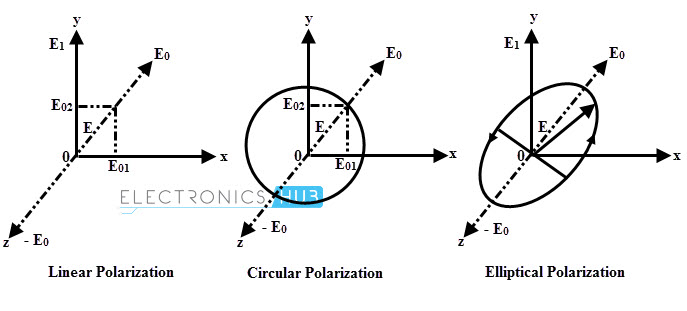
The polarization is nothing but a way in which an electric field varies with magnitude and direction. The polarization can be linear, or circular, or elliptical polarization. Let us consider that E ̅x and E ̅y are the electric fields directed along the x- axis and y-axis respectively, and also E ̅ be the resultant of E ̅x and E ̅y.
Linear Polarization
If an electric field of an EM wave is parallel to the x- axis, then the wave is said to be linearly x- polarized. A straight wire antenna parallel to x-axis could generate this type of polarized wave. In a similar way, y-polarized waves are generated and defined along the y-axis.
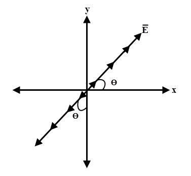
Suppose E ̅ has both E ̅x and E ̅y components which are in phase having different magnitudes. The magnitudes of E ̅x and E ̅y reach their maximum and minimum values simultaneously as E ̅x and E ̅y are in phase. So at any point on the positive z axis, the ratio of magnitudes both the components is constant.
Therefore, the direction of the resultant electric field E ̅ depends on the relative magnitudes of E ̅x and E ̅y. Thus the angle made by the E ̅ with x-axis is given by
ϴ = tan-1 Ey / Ex
Where Ey and Ex are the magnitudes of the E ̅y and E ̅x respectively.
With respect to time, this angle is constant and hence the wave is said to be linearly polarized. Therefore, the polarization of the uniform plane propagating in a z- direction is linear when E ̅x and E ̅y are in phase either with unequal or equal magnitudes.
Circular Polarization
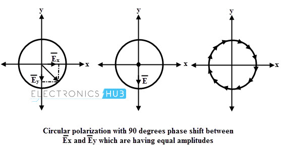
If the two planes E ̅y and E ̅x (which are orthogonally polarized) are of equal in amplitude but has 90 degrees phase difference between them, then the resulting wave is circularly polarized. In such case at any instant of time, if the amplitude of the any one component is maximum, then other component amplitude becomes zero due to the phase difference.
It is also described as if the amplitude of any one component gradually increases, then amplitude of other component gradually decreases and vice-versa. Thus the magnitude of the resultant vector E ̅ is constant at any instant of time, but the direction is the function of angle between the relative amplitudes of E ̅y and E ̅x at any instant.
If the resultant electric field E ̅ is projected on a plane perpendicular to the direction of propagation, then the locus of all such points is a circle with the center on the z- axis as shown in figure.
During the one wavelength span, the field vector E ̅ rotate by 360 degrees or in other words, completes one cycle of rotation and hence such waves are said to be circularly polarized.
Circular polarization is generated as either right hand circular polarization (RHCP) or left hand circular polarization (LHCP). RHCP wave describes a wave with the electric field vector rotating clockwise when looking in the direction of propagation.
For a LHCP wave the vector field rotates in anticlockwise direction. Therefore, the polarization of a uniform plane wave is circular if the amplitudes of two components of electric field vector are equal and having a phase difference of 90 degrees between them.
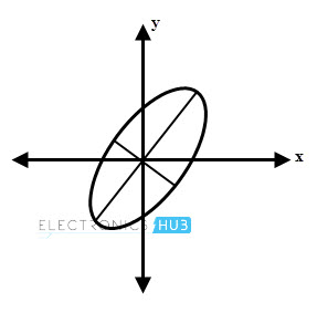
Elliptical Polarization
In most of the cases, the components of the wave have different amplitudes and are at different phase angles other than 90 degrees. This results the elliptical polarization. Consider that electric field has both components E ̅x and E ̅y which are not equal in amplitude and are not in phase.
As the wave propagates, the maximum and minimum amplitude values of E ̅x and E ̅y not simultaneous and are occurring at different instants of the time. Thus the direction of resultant field vector varies with time.
If the locus of the end points of the field vector E ̅ traced then one can observe that the E ̅ moves elliptically on the plane. Hence such wave is called as elliptically polarized.
Propagation of EM Waves in Different Mediums
In electromagnetic fields, the materials are classified as conductors, dielectrics and lossy dielectric. The electrical parameters such as µ, є and σ are the variable parameters that decide the type of medium. Different materials affect the materials differently.
Suppose if we pass through a tunnel or under the bridge, our radio ceases to receive the signals and also compared to the day, during the night time, we will experience a better reception of radio signals. Thus the waves are affected by the materials or environmental conditions.
So it is necessary to know the propagation of electromagnetic waves in order to choose the appropriate values of frequency, power, type of wave and other parameters needed for the design of applications include transmission lines, antennas, waveguides, etc.
Consider the waves obtained for a medium from equations 5 and 6 as
∇2 E ̅ = µ σ × ∂ E ̅/ ∂t + µ є (∂2 E ̅ / ∂t2)
∇2H ̅ = µ σ (∂ H ̅ / ∂t) + µ є (∂2H ̅ / ∂t2)
Both electric and magnetic fields are varying with time for a uniform plane wave. Then, the partial derivative with respective time can be replaced by jw. Thus, the electric and magnetic fields can be written as
∇2E ̅ = µ σ × (jw E ̅) + µ є (jw)2 E ̅
∇2E ̅ = [jwµ (σ + jw є)] E ̅
Similarly
∇2 H ̅ = [jwµ (σ + jw є)] H ̅
The above two equations are called as wave equation in a waveform. In the above equations the terms inside the bracket is same and properties of the medium through which the wave is propagating is represented by this term. This term is equal to the square of a propagation constant ɣ. Then the wave equations becomes
∇2 E ̅ = ɣ2 E ̅
∇2 H ̅ = ɣ2 H ̅
In terms of the properties of the medium, the propagation constant is given as
ɣ = √[jwµ (σ + jw є)] = α + j β
In general, the wave gets attenuated when it travels through a medium, hence the amplitude of the wave get attenuated. This is represented by the real part of the propagation constant and it is given by
α = w √ ((µ є / 2) √ (1 + (σ / w є) 2)) – 1)
Similarly, the phase change occurs in a wave when it propagates through a medium. This phase change is represented as imaginary part of the propagation constant and is given as
β = w √ ((µ є / 2) √ (1 + (σ / w є) 2)) + 1
And also the intrinsic impedance of a medium can be expressed as
η = √[(jwµ) / (σ + jw є)]
Uniform Plane Wave in Free Space
For free space J = 0, σ = 0, є = єo and µ = µo then the properties of the propagation constant are
α = 0 and
β = w √ (µo єo)
Therefore the propagation constant is purely imaginary for free space.
Uniform Plane Wave in Lossless Dielectric
For a perfect or lossless dielectric the properties are given as, σ = 0, є = єo єr and µ = µo µr. In both free space medium and lossless dielectric medium σ = 0, so the analysis of the wave propagation is much similar in both cases. But as the permeability and permittivity values are different then expression in both cases gets varied.
The Velocity of propagation, v = (1/√(µ є))
= (1/√( µo µr єo єr)) = 1/(√( µo єo) √ (µr єr))) = 1/(√( µo єo)/ √ (µr єr)))
Therefore v = c/ √ (µr єr) m/s
The propagation constant,
ɣ = √[jwµ (σ + jw є)] m-1
By substituting σ = 0, є = єo єr and µ = µo µr in the above equation for a perfect or lossless dielectric, we get
ɣ = +/- jw √(µє) m-1
And also attenuation constant, α = 0
The phase constant,
β = w √ (µ є) rad/m
Intrinsic Impedance,
η = √[(jwµ) / (σ + jw є)] ohms
= √(µo/ єo) √(µr/ єr)
= η o√(µr/ єr)
η = 377√(µr/ єr) ohms
Uniform Plane Wave in Lossy Dielectric
A lossy dielectric is a poor insulator, in which free charges conducts to some extent. It is an imperfect conductor and imperfect dielectric (which is a partial conducting medium) with σ ≠ 0.
The propagation constant is given as
ɣ = √[jwµ (σ + jw є)]
Rearranging the terms, we get
ɣ = √[jw є (1 + (σ/ jw є)) jwµ]
Therefore, ɣ = α + j β= jw √µє √ (1 – j (σ/ w є))
The above equation gives the propagation constant for lossy dielectric medium which is different from lossless dielectric medium due to the presence of radical factor. The attenuation constant α and phase constant are calculated by substituting the values of w, µ, є, and σ in the above equation.
The attenuation constant α indicates the certain loss of the wave signal in the medium and hence this type of medium is called as lossy dielectric.
And also due to σ ≠ 0, the intrinsic impedance becomes a complex quantity and is given as
η = √[(jwµ) / (σ + jw є)]
η = |η| ∠ Өn Ohms.
Because of the complex quantity, η is represented in polar form as shown in the above equation where Өn is the phase angle difference between electric and magnetic fields. Thus, in lossy dielectric medium there exist a phase difference between the electric and magnetic fields.
The intrinsic impedance can be expressed as
η = √[(jwµ) / (σ + jw є)]
= √[(jwµ) / jw є (1 + (σ/ jw є)]
η = (√ (µ/ є)) (1 / √ (1 – j (σ/ w є)) ohms
And the angle Өn is given as
Өn = ½ [(π/2) – tan-1 (w є/ σ)]
This angle depends on the frequency of the signal as well as properties of the lossy dielectric medium. Then, w becomes very small for a low frequency signal. Thus, the phase angle is given as
Өn = (π/4)
For very high frequency signal, w becomes very large then,
Өn = 0
So the range of Өn of a lossy dielectric for complete frequency range is 0 Өn (π/4).
Applications of Electromagnetic Waves
In general, a wave phenomenon constitutes both time varying electric and magnetic fields. Some of the applications where the electromagnetic waves can be encountered are given below. In addition to the below application areas there are many other applications where the knowledge of the electromagnetic waves is profoundly used.
Transmission Lines
In case of power transmission at low frequencies, electrical parameters like resistance, capacitance, inductance, etc are enough to characterize the complete electric circuit. In such circuit analysis, the physical size of electrical components is not considered and simple Kirchoff’s laws are enough to analyze the circuit.
However, if the frequency is increased, the size of the physical parameters must be considered and also space starts playing a role in the analysis of the circuit.
In such transmission the voltages and currents are exists in the form of waves. This type of approach for analysing the circuit with inclusion of space consideration is called as a transmission line approach.
Antennas
An antenna is one of most important devices in the communication system, although it appears as a passive looking device. It can efficiently launch and receive electromagnetic waves. Several types of antennas have been in use for serving different applications.
With the advancements in the mobile communications, compact, multi-frequency and efficient antennas are developed during recent years. By using the power ranging from a few watts to Mega watts, the communication is established by these antennas.
Mobile Communications
The understanding of radio environment requires the knowledge of electromagnetic wave propagation. In a cellular system, different frequency reuse schemes are employed depends on the signal strength variation as a function of distance. One of the major important aspect of the mobile communication is fading.
Thus, for correctly predicting the behavior of the fading, signal processing algorithms need the knowledge of the radio environment. Hence the electromagnetic waves and its analysis plays key role in mobile communication systems.
Fiber Optic Communication
A high speed and efficient long haul communication use a variety of fiber optic devices which are developed by employing the complex phenomena of electromagnetic waves. This communication is the modern form of guided wave communication.
For the investigation light propagation in the optical fibers electromagnetic theory is used. Due to the direct consequence of the direct consequence of the wave nature of light results a modal propagation inside an optical fiber. Also for analysing the photo and laser detectors, the electromagnetic wave theory is very important.
Electromagnetic Interference (EMI) and Compatibility
In general, an electric circuit tends to give electromagnetic radiation, especially when they are switching heavy currents. This radiation may interfere with other parts or elements in the network, thereby affect the overall circuit performance.
Example case is SMPS and high speed digital circuits produce a considerable electromagnetic interference. Mostly shielding circuits are used for protecting the circuits from EMI. Thus the proper design of such EMI shields requires the knowledge of electromagnetic waves.
Radio Astronomy
The radio astronomy is a combination of physics and electronics engineering. It is one of the major important areas where understanding of the electromagnetic waves is necessary. In astronomy, the observations of the sky are carried out at radio frequencies.
These RF signals are very weak in nature and thus sate of art communication receivers and antennas are used to detect such signals. Therefore, in radio astronomy all aspects of electromagnetic waves are employed.

One Response
Clearly explained. I loved it.